Normal Distribution
Basics of Probability
Definition of Probability: The chance of an event occurring, represented as a proportion between 0 and 1, or as a percentage from 0% to 100%.
Example: Probability of rain or a cyclone.
Importance of Probability: Often, we cannot gather data from an entire population, so we rely on samples to represent the larger group. Understanding probability distributions is fundamental in statistical analysis.
Probability Distribution and Normal Distribution
Probability Distributions: Used to represent the likelihood of occurrences of different outcomes. These can be either theoretical or empirical.
Normal Distribution: A specific type of distribution that is symmetric and bell-shaped. Characteristics include:
One peak (mode) at the center.
Symmetric bell shaped Mean, median, and mode are equal. Half scores lie below the curve and half above the curve.
Total area under the curve equals 1 (or 100%)
Assumptions: Many statistical tests assume that collected data fits a normal distribution.
Calculating Probability
Probability Formula:
Probability = (Number of favorable outcomes) / (Total number of possible outcomes)
Example: Tossing a coin has a probability of getting heads or tails as 0.5 or 50%.
Example: Rolling a die, probability of landing on a 4 is 1 out of 6, or approximately 16.7%. Rival
Empirical distribution - distribution based on data
Probability distribution- based on theory and specified by mathematical formula/function
used to calculate theoretical probability
Exists for both continuous and categorical data
Z Scores
Z Scores: Measures how many standard deviations an element is from the mean. Calculation is:
Z = (Observed score - Mean) / Standard deviation
Purpose: Z scores help in standardizing scores from different distributions for comparison. A Z score of +1 means one standard deviation above the mean, while -1 means one standard deviation below.
Without a-score, we cannot answer questions until we find the average mark and SD
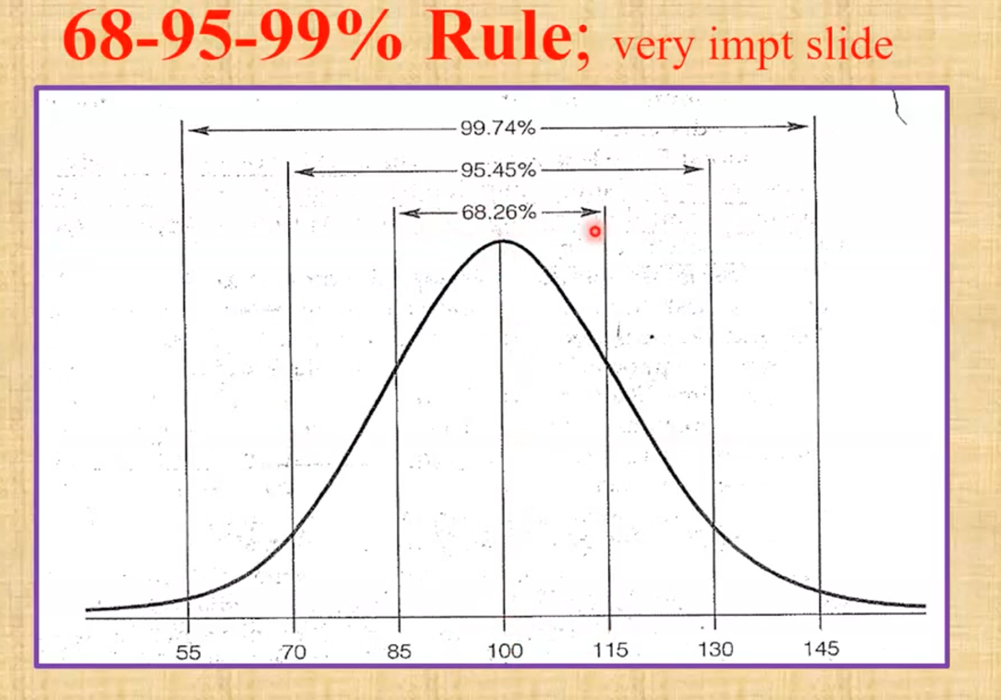
Characteristics of Normal Distribution
The bell shape of normal distribution illustrates that:
68.3% of data lies within one standard deviation from the mean.
95.4% lies within two standard deviations.
99.7% lies within three standard deviations.
Example: Sampling IQs from a population where the mean is 100 and standard deviation is 15.
68% of scores will be between 85 to 115 (mean ± 15).
95% will be between 70 to 130 (mean ± 30).
99% will be between 55 to 145 (mean ± 45).
 Testing for Normality
Eight methods to assess normality:
Comparing means, medians, and modes.
In a normal distribution, they should be very close.
Skewness and Kurtosis.
Both should be approximately 0 for normal distribution.
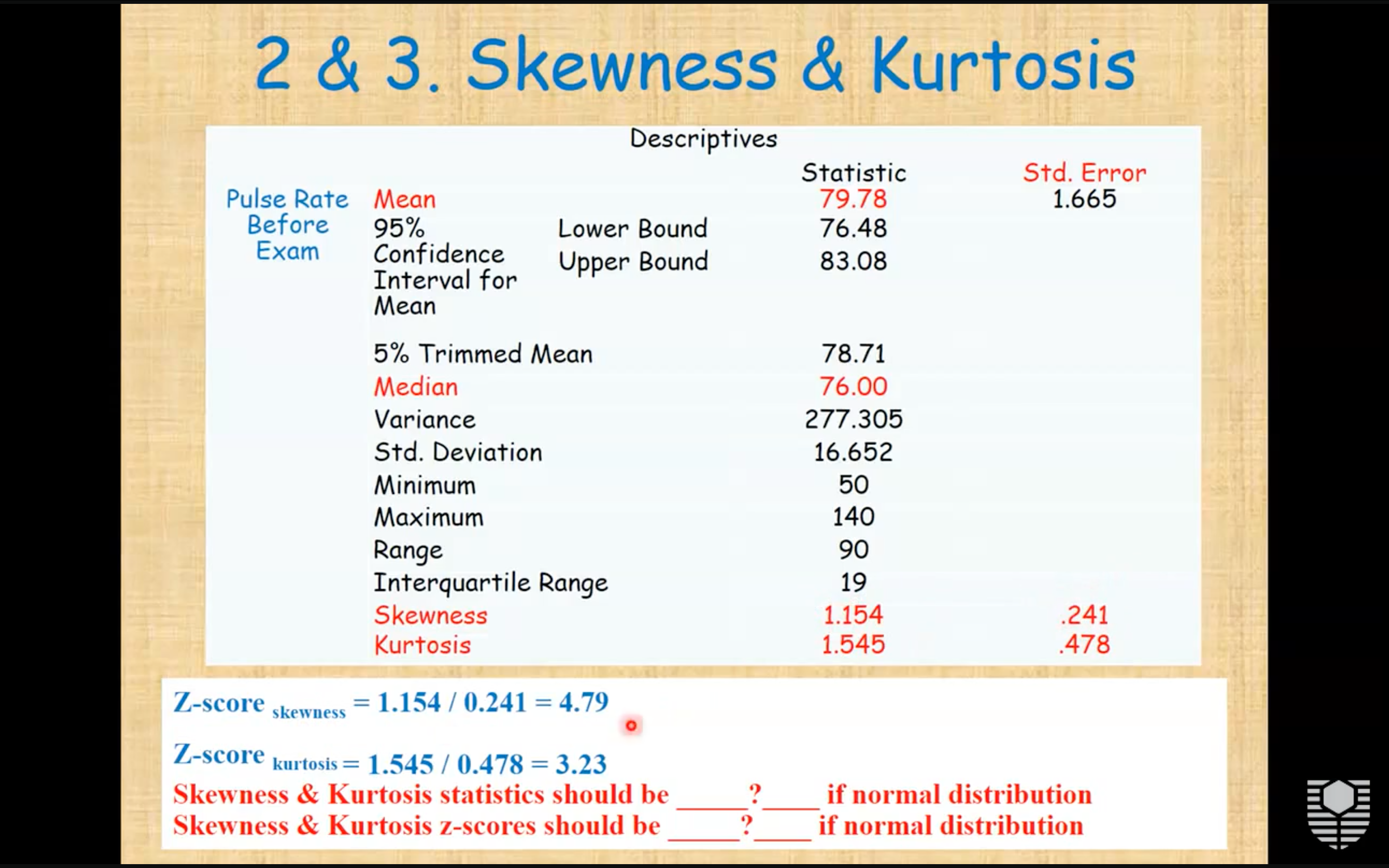 - both zero
- within plus minus 1.96
Shapiro-Wilk Test.
Tests if the sample comes from a normally distributed population; significance <0.05 indicates violation of normality.
Histograms.
Visual representation; should appear symmetric for normal distribution.
Box Plots.
Useful for visualizing median and identifying outliers.
Normal Probability Plots.
Points cluster close to a straight line if data is normal.
Detrended QQ Plot.
Should show similar distribution of points above and below a central line.
Empirical Rule (68-95-99.7 Rule).
Stem and Leaf
Applying Z Scores and Normal Distribution
Example scenarios:
If average weight in a population is 65kg with a standard deviation of 5kg, approximately 68% will weigh between 60kg to 70kg (one standard deviation).
For two standard deviations, weight will range between 55kg to 75kg with about 95% of the population falling within this range.
Conclusion
When assessing for normality, all eight methods must be examined together to draw a final conclusion about the sample data distribution.
SPSS can be utilized for visualizing these distributions and conducting the necessary tests for interpretation.