PS225 T1 W1 - Quant Methods as Estimation/Single Sample T-test, Paired T-test, Independent T-test - Lecture and Demo notes
Lecture Notes
Quantitative research: Estimation
When conducting quantitative research (The general idea of quantitative research):
We have a conceptual research question about the universe
In Psychology, the part about the universe we care about is minds and behaviour
We turn it into a question about a number that describes the universe (minds and behaviour). This allows us to quantify our question.
We use data to estimate that number
We try to use that estimate to answer our question
To answer our question, we need to make it about numbers:
E.g. Are dogs generally left-pawed, generally right-pawed, or neither?
E.g. How often do dogs choose to use left (or right) paws?
Is our numerical estimate good?
If we are using a numerical estimate to answer our research question, we want that number to be “good” in two senses:
Validity - are we estimating the right thing to answer our question?
Reliability - will we get the same estimate if we measure again?
Estimates - Validity: Things that affect the validity of our numerical estimate
Are the outcome variables we are measuring relevant to the question?
It would not be correct if, in our initial research question, we wanted to find out about the number of times a dog used either paw, but then the outcome variables we measured were the speeds at which a dog used either paw.
Are the “predictors” the real explanation of what happened?
Could relationships involving predictors be attributed to other causes?
Basically meaning, when trying to predict the relationship between variables, are the “predictors” the real explanation/cause of the outcome? Or is there other unseen “predictors”/variables that have not been taken into consideration by the experiment?
Does the sampling scheme (participant tool?) reflect the population we were asking about?
Is the pool of data we are getting represetative of the people we are looking into, or the situations that we care about? In other words, does the numerical estimate have “external validity”?
Estimates - Reliability: This that affect the reliabiity of our numerical estimate
We will never get the exact same answer if we were to measure again because we rely on samples to get estimates, however, of we get a significantly different answer every time, that how do we know what is true?
Samples of the possible people that we could study within the parameters of our study, and so by chance, it is possible that we may get some people who do not reflect the average.
Samples of occasions - even when using the same people more than once, these people don’t behave the same all the time
A different sample will give a different estimate - variability
A variable estimate might be off a little or a lot; we don’t know for sure. The variability can pose a problem when we are trying to make decision from our data because we know that it is not exactly represent the whole possible data, and instead just representing small part of it.
A possible experiment:
Select random dogs (sampling: different dogs are different)
Do something to make them use their preferred paw
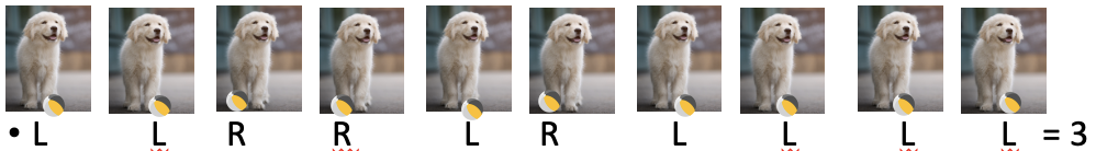
E.g. Roll a ball towards them and see which paw touches it first
Don’t let them copy each other - this is because we want the participants to behave independently.
E.g. Roll a ball to a dog 10 times - which paw touches the ball first? We can give each dog a “right-handedness” score: # of times used /10
10 = a very right-pawed dog; 0= very left pawed dog; 5 = equally left and right
There’s also sampling here - different trials
Just because its the same participant, doesn’t mean you get the same data from them every time.
If we did this again, 10 times with the same dog, this does not mean that we will get the same result.
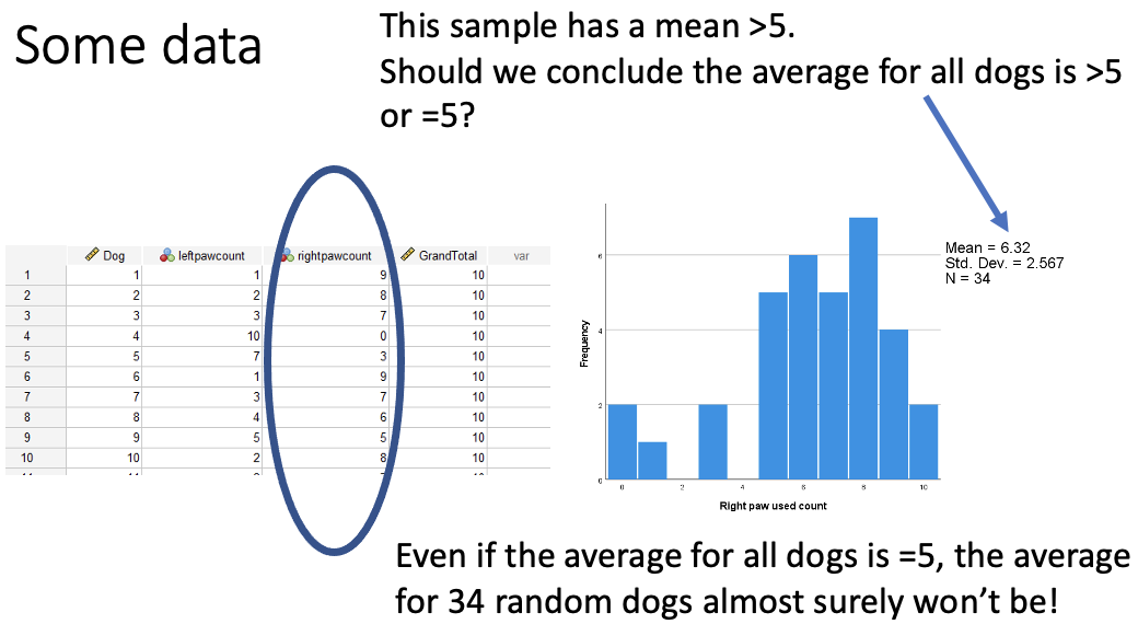
Whilst the average here is above 5, but we know that our sample is random and that another sample is likely to be different. Also, is this different enough from five to believe that the average for all diogs is greater than 5, or if it could still be 5 when adding more samples.
This is a problem with data as it doesn’t tell us what the whole population is like, but instead it just tells you what your sample is like.
We need to make an inference from our data about the population at large, and there are two closely related approaches to this:
Two related approaches:
Hypothesis tests
Asks a yes/no question about a value we are trying to estimate
Confidence intervals
E.g. Is the average 5 or is it not?
Express our uncertainty around the estimate
This expresses our uncertainty in the estimate, whilst also giving numerical values that could be where initial numerical value is that you’re trying to find.
Statistical hypothesis test = A rule to decide between hypotheses
Null hypothesis - the average is 5
Alternative hypothesis - the average is not 5
From Hypotheses to tests
Our test can’t give the right answer every time
Typically, both hypotheses say the data we see are possible
A good test controls how often we are wrong (error rates)
As much as is possible
To make such a calculation possible, we cannot do this from the hypothesis alone, but we need to make some assumptions that enable the maths, and how good our estimates about the errors are and how good our assumptions are will determine whether our error rates are true or not
What is meant by assumptions here are things that “go into the maths” that express facts about how the data was collected, and things that are estimates of how the data is distributed.
Facts aboyt how the data were collected
Guesses about how the data are distributed
Tests compare models = hypotheses + assumptions
Putting together a hypothesis and the assumptions makes a mathematical/statistical model. This means that our two hypotheses turn into two models, whilst the assumptions are the same between the two models, and so we make a decision between the two hypotheses, assuming the assumptions are true.
A common assumption: Normal Distribution
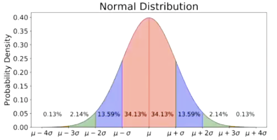
This is the default “guess/assumption” in data analysis for continuous variables
This is just saying that any number is possible but most of them are close to the average.
This depends on the mean (μ) and the variance (σ2). When a random variable X is drawn from this diostribution, this fact is often abbreviated: X~N(μ, σ2)
Mu (μ) represents the mean, the sigma (σ) represents the standard deviation, how spread out away from the mean things are. The square of the standard deviation is the variance. When we say that something is normally distributed, the abbreviation is: X~N(μ, σ2)
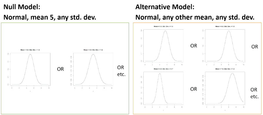
When this is applied to our question of the average righthandedness score in dogs being 5, the null hypothesis (model) will say that the mean is 5, but does not say anything about the standard deviation. Where as the alternative hypothesis will say a different mean and a different standard deviation
When looking to use the best possible test in this istuation, we come up with the single sample T-test.
Single-Sample T-test
This is used for these type of questions that ask “is the average different from an ideal/theoretical value M (that was known in advance)?”
Basically saying “is the mean that we’re measuring the same or different from a number that we had in mind from the start?”
The estimate - is the average of the sample
The assumptions we’re using is that there is a normal distribution that all these data come from, and they are coming from this distribution independently. No one data point has any reason to be more similar or different than any other data point.
Keep it so that there are no clusters of data. For example, make sure that you haven’t measured the same dog twice. In SPSS, you should only have one subject’s data per row, and each subject should only be one row.
Examples of uses for Single-sample T-tests
The kind of things that we may use a single sample t-test for are:
When things have a score, and the score has enough different values, and not just 0 and 1 and we may want to compare the score to something such as:
Guessing - e.g. did children learn (anything about) the words in a forced-choice test?
Basically, when you have attempted to teach kids something and want to see if they’ve learned anything, they could be given a forced-choice test/multiple choice test. If there are 4 options for each question, then we’d expect them to get a quarter of the questions correct.
Measuring preference (as in the dog pawedness example):
E.g., do dogs prefer to use their right paw (when tested repeatedly) or their left paw? if they don’t prefer, then we expect them to use one paw 5/10 times. In these situations, things wil be approximately normally distributed, not perfectly, but enough so for the use of the test.
Expected count: m = number of choices/number of options
Doing a t-test
The general idea of a single sample t-test is that we have to pick a type 1 error rate.
A type one error is when looking at the data, we believe that there is a significant effect, but there isn’t. Essentially meaning, we failed to choose the null hypothesis when we actually should have.
We usually use 0.05 as the significance level (aka alpha [α] level)
What we do to achive a test that has this error rate is: you compute your T-statistic, then to implement this particular error rate…:
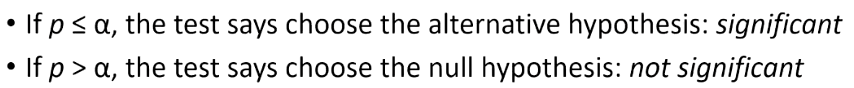
1. Work out the P value from the T statistic (spss does for you, in the “Sig. (2-tailed)” column). If the p-value is greater than the significance level (alpha [α] level), fail to reject the null hypothesis.
T-statistic
The t-statistic can be calculated as
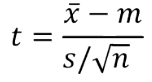
x̄ = this is the observed mean.
m = is the mean that you are planning to compare to
s = observed standard deviation
n = number of observations
estimtaed/observed difference from m = this is how big the difference is of our observed mean from the one we thought it should be. E.g. if we observed an average dog score of 6.2 and we were thinking 5 in advance to the study, that is a difference of 1.2. That is how far off what we expected.
s/ √n = the standard error, which is how much variability we infer there should be around that mean.
The data was not going to be exactly on the number we expected, 5. This is working out a big and small variation around this value.
Big values of t reflect a large difference, because the difference is on the top, relative to what we might expect (which is on the bottom.
Confidence intervals
Confidence intervals are an alternative way of looking at the link between our estimates and our decisions about hypotheses
CIs for some tests can be more easily calculated than p or critical values.
Rther than a yes/no decision on a singlue value, m, a CI identifies a range of ‘plausible’ values of the overall mean, m.
This means that some values that are “close enough” to the observed x̄.
The wider we make our confidence intervals, the more likely we are that it contains the correct value, and the narrower we make the confidence intervals, the less likely that they contain the correct value.
This means that confidence intervals also have error rates. A confidence interval that is contstructed to miss the the right value 5% of the time is knwon as a 95% confidence interval. The 95% CI is the CI that has an error rate of α = 0.05
These can then be used to do the same thing as a hypothesis test by thinking of the CI as “the range of calues that our observed value is not significantly different from.” - These are the values that if we had chosen them for our hypothesis, we would have made a not significant result for. This means that if 0 is in the CI then what we have observed is not significantly different from 0.
Paired (repeated measures) t-test
This is used for the type of question where instead of one meausrement per participant, we have 2 (or other situations where we have pairs of values and we want to know if they’re different from each other).
Estimate: difference between the two means from our sample - is the difference here 0 or not.
Assumptions - the difference between the pairs follow a normal distribution
The paired t-test simply works out the difference for each pair and does the one-sample t-test on those differences.
Example uses of paired t-test
Within subjects experiments with 2 conditions
E.g. compare paw speed in a left-paw condition to that of the same in a right paw condition to test pawedness
Can be used for comparing two different but similar measures for two subjects
E.g. what oercentage lecture are attended, what percentage of seminars are attended.
Things where there are a natural pairing of subjects
E.g. Does the eldest sibling have better social skills than the youngest sibling? (where siblings come in pairs - i.e., for every eldest sibling in the data set, there is a youngest sibling from the same family)
Independent measures t-test
This is used instead for when you have two groups that give two means, but now we need to assume that each groups data has a normal distribution, and still that every data point is not related to one another except by what group they are in.
Example uses of independent t-test
Between subjects experiments with two conditions
e.g. let half dogs use their left paw and the other half use their right paw and then compare the right paw dogs to the left paw dogs.
Video demo notes
Single Sample T-test - SPSS
To perform a single sample t-test in SPSS:
Analyze → compare means → one sample t-test.
Next, the screen bellow will show:
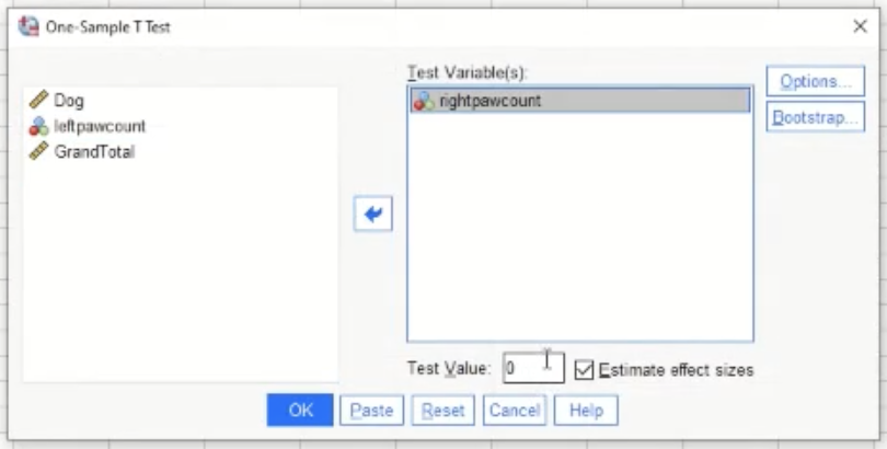
Move the variable that you are interested in into the box on the right.
The test value is the mean that you are comparing to (in the dog example from earlier, the test value would be 5)
Next you will get the output table as so:
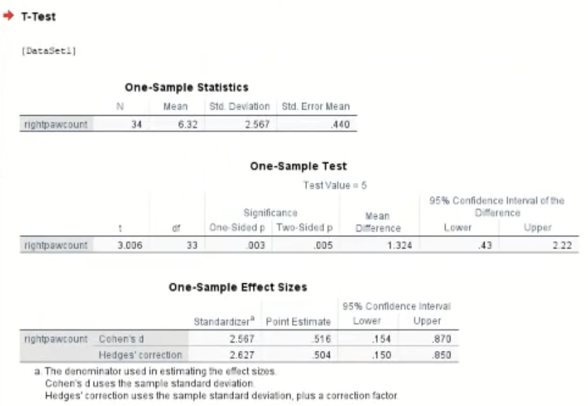
Reporting a single sample T-test
Once gaining the output table in SPSS, interpret the stats:
Right paw counts (M = 6.32) were significantly higher than the expected chance value (5.0), t(33) = 3.01, p = .005
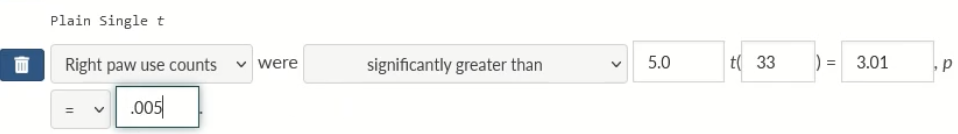
Above is how it should look in the assessment system.
Confidence Intervals in Excel
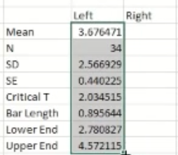
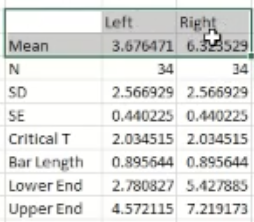
Once you have the data, re-represent the data as shown below:
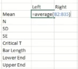
Mean (M)To get the Excel system to do the Average calculation for you, type in “AVERAGE” in the cell
N = (number of items) - to get the excel system to count this for you, type “COUNT” in the cell
Standard Deviation - To get excel to do this for you, type “STDEV” in the cell.
Standard error - this is the standard deviation divided by square root of N
Critical T - for Excel to do this for you, type “=t.inv.2t(0.05, (degree of freedom))
Degree of Freedom is N-1
Bar Length - multiply the values of Critical T and SE in otder to have the right number
Lower end - the value that you have in the “Bar length”, subtract this figure from the mean in order to gain the Lower end
Upper end - Add the value that you have in the Bar Length cell to the mean value in order to get the upper end value.
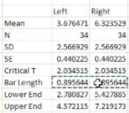
From here, since the right side is empty, highlight all of the values that you input as shown below:
Then, press and hold that little green square ………..^ and drag it over to the right sided column and Excel will fill in the data appropriately.
Now all that is left to do is to get a graph showing the confidence intervals visually. Highlight the section shown below:
Then press “insert” → 2d bar graph
Then to add the confidence intervals to the graph, hover over the graph and click the “+” icon that shows, then click the “error bars” option. Then click the “more options’ option. On the right side of the screen, there should be an option that says “custom”. Select this. Then press, “specify value”. Then in the pop-up that appears, copy the values in the bar length cells for left and right like shown below:
Copy these values into both the positive error value box and the negative error value box.
If you are required to make a bar graph that includes error bars from these numbers you have calculated, the error bars from some of the bars in the graph may be smaller than others. There may be 2 reasons for this:
There are more participants one one group than there are in the other group. Standard error (SE) is calculated as: SE = SD/ √N. As the number of participants in the group increases (N gets bigger), the denominator (√N) also gets bigger, which makes the standard error smaller. A smaller SE leads to a shorter error bar.
The standard deviation for one group is smaller than the standard deviation for the other group, meaning the error bar will be smaller. Standard error is directly proportional to standard deviation. This means that a smaller SD (meaning less variability in the data) means that the SE is also smaller. Again, smaller Standard Error means the error bar will be smaller.
Paired (repeated measures/within-subjects) T-test - SPSS
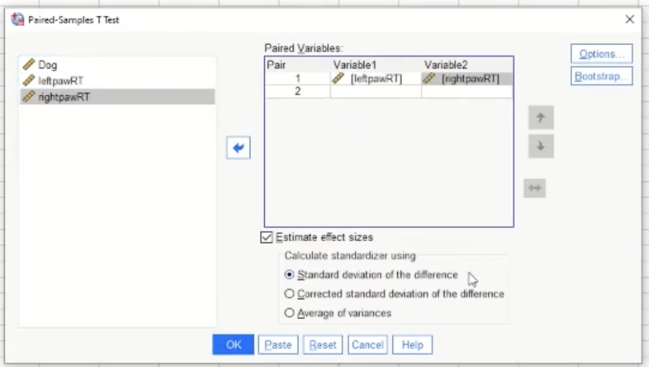
To perform a paired T-test: Analyze → compare means → paired samples t-test
Then in the pop up, move the variables that you are interested in comparing like shown below:
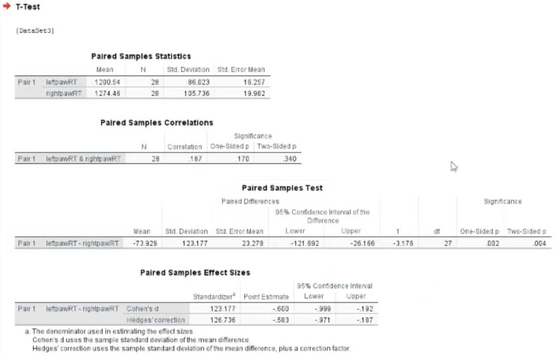
This will then give you the output table as below:
Reporting a Paired t-test
Once gaining the output table: interpret the stats:
Response times in the left paw condition were significantly shorter than those in the right paw condition, paired t(27) = 3.18, p= .004
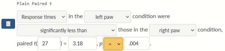
Above is how it should appear in the assessment system
Independent measures (between-subjects) T-test
When conducting an independent measures t-test, the data may look like:
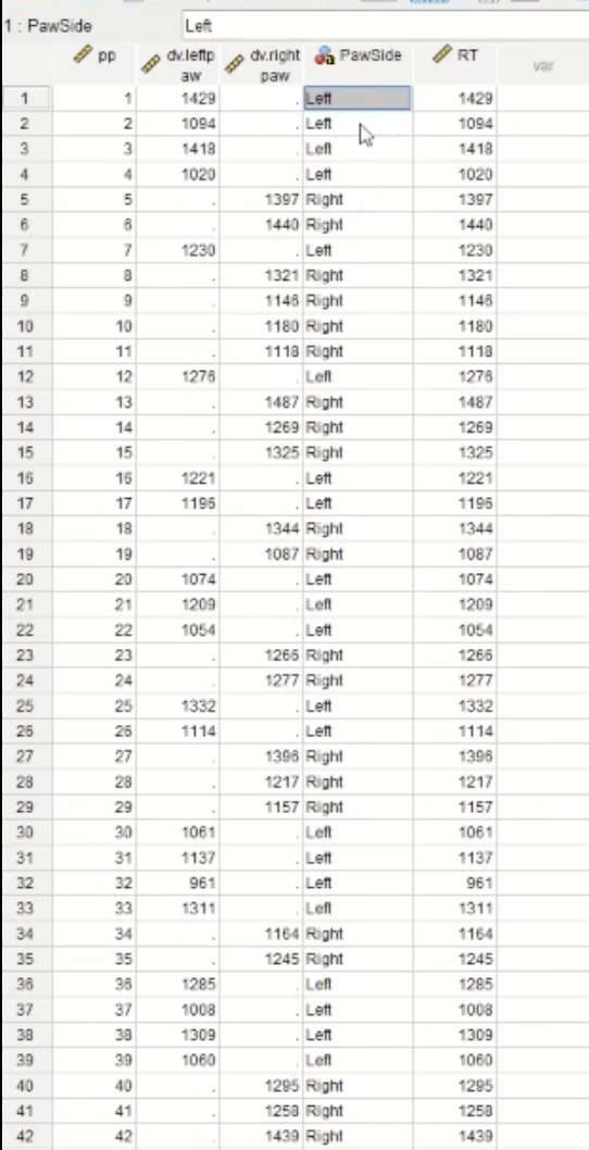
The column titled ‘PawSide’ will not work in its current state when doing the t-test as it is currently in “string form”. In order to make it so that the column will be in the proper form, you will need to “recode” it:
Transform → Automatic Recode
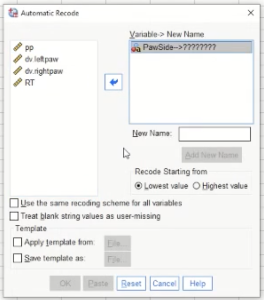
This is the pop-up after selecting Automatic Recode. Move the variable that you are concerned with into the box on the right, in this case, “PawSide”. Give it a new name in the designated box. Once OK is selected, below shows what follows:
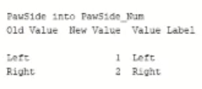
This is showing what the values in the column looked like before when they were in string form, and this is what they look like now when they are in the right form. 1=left, 2=right.
Now, to conduct the T-test: Analyse → compare means → independent samples t-test. Below shows the pop-up:
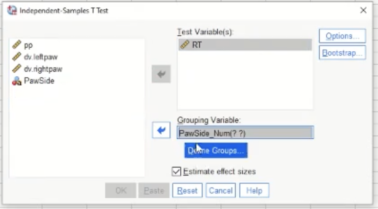
“Test variable” is the dependent variable or the outcome variable. Here we are comparing the means in reaction times (RTs) of the two groups
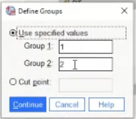
This is the pop-up when “define groups” is pressed. Left is 1, right is 2 - so the default is fine here.
Below shows the output table:
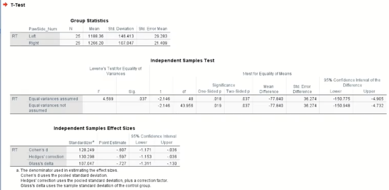
Reporting an Independent measures T-test
Once gaining the output table - interpret the stats:
Reaction times (RTs) in the left paw condition we significantly shorter than those in the right paw condition t(48) = 2.15, p = .037
This is what it should look like in the assessment system: