Matrix Applications Table of Contents Significance of Matrix Operation Graph Representation using Matrices Linear Transformations Real-World Applicati
Matrix Applications
Table of Contents
Significance of Matrix Operation
Graph Representation using Matrices
Linear Transformations
Real-World Applications
Significance of Matrix Operation
Computer Science and Engineering
Physics and Mathematics
Economics, Finance, and Game Theory
Environmental Science and Biology
AI/ML, and Robotics
Matrix Operations in CSE
Graph Theory and Networks
Graph Representation:
Adjacency Matrix: Represents graph connectivity.
Path Matrix: Shows reachability between nodes.
Algorithms:
Path finding and Network Analysis use matrix operations for tasks like shortest path and flow analysis.
Computer Graphics and Image Processing
2D/3D Transformations:
Matrices apply scaling, rotation, and translation to objects.
Image Filtering:
Matrix convolution is used for blurring and edge detection.
Rendering:
Matrices control perspective and angles in 3D graphics.
Control Systems
Kinematics:
Matrices compute motion and orientation of robotic systems.
State-Space Representation:
Matrices model multivariable systems for stability and control analysis.
Physics and Mathematics
Quantum Mechanics:
Matrices in Operators: Used for quantum state transformations and eigenvalue problems.
Linear Algebra in Mechanics:
Inertia Tensors and Rotation Matrices: Applied in rigid body dynamics.
Stress-Strain Analysis: Matrices model material behavior under stress.
Relativity and Electromagnetism:
Lorentz Transformations: Matrices describe changes in space-time.
Minkowski Spacetime: Used in special relativity.
Maxwell’s Equations: Represented in matrix form for field equations.
Numerical Methods and Simulations:
Solving Systems of Equations: Matrices are used to find solutions efficiently.
Finite Element Methods (FEM): Matrices model complex physical systems.
Differential Equations: Matrix operations solve differential systems.
Economics, Finance, and Game Theory
Economic Models:
Input-Output Models: Matrices represent economic interactions between sectors.
Production Systems: Matrix-based analysis of resource allocation.
Portfolio Optimization:
Covariance Matrices: Used for asset risk analysis and optimal portfolio construction.
Game Theory:
Payoff Matrices: Represent strategies and outcomes.
Nash Equilibrium: Matrices help in finding optimal strategies.
Optimization Problems:
Linear Programming: Matrices are used to solve optimization problems in various fields.
Environmental Science and Biology
Ecological and Population Models:
Population Dynamics: Matrices model growth, predator-prey relationships, and ecosystem interactions.
Climate and Weather Modeling:
Environmental Systems: Matrices simulate climate patterns and predict changes.
Bioinformatics and Genetics:
Genetic Sequence Analysis: Matrices represent DNA/protein sequences and their similarities.
Systems Biology:
Biological Networks: Matrices represent metabolic and signaling networks for pathway analysis.
Machine Learning, AI, and Robotics
Neural Networks and Deep Learning:
Forward & Backward Propagation: Matrices are used in computations for weight updates and error backpropagation.
Dimensionality Reduction:
PCA & Matrix Factorization: Matrices reduce feature spaces and simplify data representations.
Computer Vision and Object Recognition:
Matrix Transformations: Used for feature extraction, image processing, and recognition tasks.
Reinforcement Learning:
Matrix Operations: Applied in value functions, Q-learning, and policy optimization.
Graph Representation using Matrices
Introduction
A graph is a mathematical structure used to model pairwise relations between objects. It consists of:
A set of vertices (also called nodes).
A set of edges connecting some or all pairs of these vertices.
Node
The fundamental building blocks of a graph are nodes, which represent individual entities.
Nodes are also known as vertices.
We can represent a node as N or V.
Edge
Edges define the connections between nodes.
Edges are also known as arcs.
Types of Graphs
Directed Graphs
Undirected Graphs
Undirected Graphs
In undirected graphs, the connections between nodes go both ways, and one can travel along the edges in either direction.
For instance, node 0 can visit node 1 and node 1 can also visit node 0.
Directed Graphs
In directed graphs, edges have a clear direction, like one-way streets. This shows a specific flow from one node to another.
For instance, node 1 can visit node 2, but node 2 can't visit node 1.
Directed Graph vs. Undirected Graph:
Directed
Edges have direction. For instance, an edge from vertex A to vertex B does not imply there’s an edge from B to A.
The matrix may not be symmetric.
Undirected
Edges have no direction. If there’s an edge between A and B, it means there’s also an edge from B to A.
The matrix is symmetric: Aij = Aji.
Adjacency Matrix
An adjacency matrix is a 2D grid (matrix) used to represent a graph. Each cell in the matrix shows whether there is a connection (edge) between two vertices (nodes) in the graph.
Edge between i and j: If there’s an edge from vertex i to vertex j, the matrix value Aij = 1 . Otherwise, Aij = 0.
Example - 1:
Let’s take a directed graph with vertices A, B, and C:
There is an edge from
A
to
B
,
There is an edge from
B
to
C
,
No other edges exist,
The adjacency matrix is:
A B C
A [0, 1, 0]
B [0, 0, 1]
C [0, 0, 0]
Example - 2
Let’s take a undirected graph with vertices A, B, and C:
An edge between A and B
An edge between A and C
An edge between B and C
No other edges
The adjacency matrix is:
A B C
A [0, 1, 1]
B [1, 0, 1]
C [1, 1, 0]
Multiplication in Graph Theory
What is Matrix Multiplication in Graph Theory?
Matrix multiplication helps us find paths between vertices in a graph.
By multiplying the adjacency matrix by itself (i.e., A x A), we get a matrix that shows how many paths exist between vertices of length 2.
Path finding
Multiplying the adjacency matrix by itself helps find paths of different lengths between vertices.
A2: Paths of length 2 between vertices.
A3: Paths of length 3 between vertices.
And so on…
This helps to analyze how vertices are connected through multiple steps.
Matrix Multiplication
Let’s take the adjacency matrix M of an undirected graph.
A B C D
A [0, 1, 1, 0]
B [1, 0, 1, 0]
C [1, 1, 0, 1]
D [0, 0, 1, 0]
Multiply M by itself to get M2, which shows paths of length 2.
A B C D
A [2, 1, 1, 1]
B [1, 2, 1, 1]
C [1, 1, 3, 0]
D [1, 1, 0, 1]
Each cell in M2 shows the number of length-2 paths between the corresponding vertices.
Multiply M2 by M to get M3, which shows paths of length 3.
A B C D
A [2, 3, 4, 1]
B [3, 2, 4, 1]
C [4, 4, 2, 3]
D [1, 1, 3, 0]
Each cell in M3 shows the number of length-3 paths between the corresponding vertices.
Question 1 of 3
Show AnswerSubmit
Linear Transformations
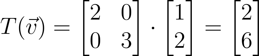
A linear transformation is a mathematical operation that modifies a vector while preserving key geometric properties like straight lines and distances.
Matrix representation: A vector is transformed by multiplying it by a matrix A:

This matrix A defines how the vector is transformed.
Types of Linear Transformations
Scaling
Rotation
Reflection
Shearing
Scaling:
Scaling is a type of linear transformation that stretches or shrinks a vector along certain directions (axes).
In other words, scaling changes the size of a vector by multiplying its components by a scale factor, either enlarging or reducing it along specified axes.
Mathematical Representation
For a 2D vector
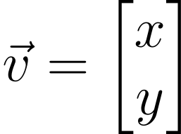
scaling is done by multiplying it with a scaling matrix:
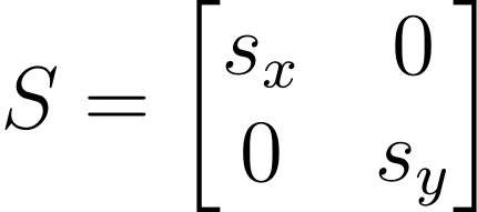
where:
sx is the scaling factor along the x-axis.
sy is the scaling factor along the y-axis.
How It Works
The transformed vector is:

where:
If sx > 1, it stretches along the x-axis.
If 0 < sx < 1,it shrinks along the x-axis.
If sx = 1, it stays the same along x.
Negative values flip (reflect) the vector across the axis.
Example
Let’s say:
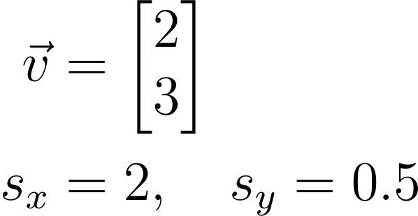
Then:
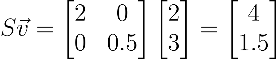
This doubles the x-component and shrinks the y-component to half.
Rotation:
Rotation is a type of linear transformation that turns a vector around the origin (0,0) by a certain angle θ.
In other words, rotation changes the direction of a vector by turning it around the origin (0,0) by a specific angle θ without changing its length.
Mathematical Representation
For a 2D vector
rotation is done using a rotation matrix:
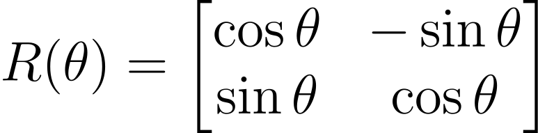
Here:
θ is the angle of rotation(in radians or degrees).
Counterclockwise is the positive direction.
How It Works
The transformed vector is:

Example
Let’s say:
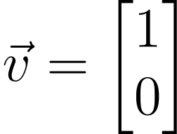
Rotate by θ = 90 = π/2 radians.
The rotation matrix:
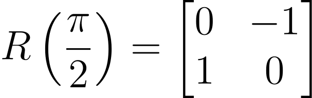
Applying it:

So the vector (1 , 0) rotates to (0 , 1).
Reflection:
Reflection is a linear transformation that flips a vector or shape over a specific line (in 2D) or plane (in 3D), like looking in a mirror.
For example, reflection over the x-axis flips the vector upside down, while reflection over the y-axis flips it left to right.
Reflection over the x-axis:
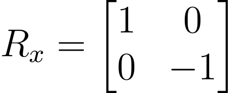
Effect:
x stays the same.
Y changes sign(flips).
Reflection over the y-axis:
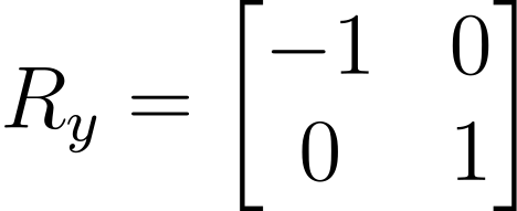
Effect:
x changes sign(flips).
y stays the same.
Reflection over the line y = x:
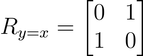
Effect:
Swaps x and y.
Example
Let’s take:
Reflection over the x-axis:
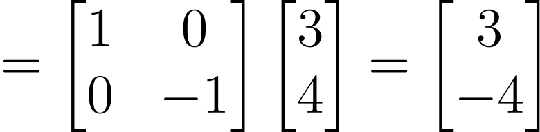
The vector is flipped vertically, but the x-component stays the same.
Shearing:
Shearing is a linear transformation that slants or skews the shape of an object along one axis while keeping the other axis fixed. It looks like pushing the top of a rectangle sideways so it becomes a parallelogram.
Unlike scaling or rotation, shearing changes the shape but preserves the area (in some cases) and keeps lines parallel.
Shearing along the x-axis:
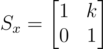
Effect:
Moves the x-component by a factor proportional to the y-component.
k is the shear factor (how much slant).
Shearing along the y-axis:
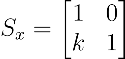
Effect:
Moves the y-component by a factor proportional to the x-component.
Example
Let’s take
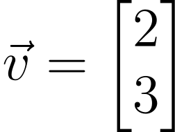
and shear factor k = 1.5 along the x-axis:

The vector’s x-value is increased based on its y-value.
Practice Problems
Question: Given a directed graph with vertices A, B, and C, and edges A → B, B → C, create the adjacency matrix.
Solution:
A B C
A [0, 1, 0]
B [0, 0, 1]
C [0, 0, 0]
Question: Given the adjacency matrix A for a graph, find the number of paths of length 2 between vertices.
[0, 1, 1]
[1, 0, 1]
[1, 1, 0]
Solution:
To find the number of paths of length 2 between vertices in a graph, you can compute A² (the square of the adjacency matrix).
The entry at position (i, j) in A² tells you how many paths of length 2 exist from vertex i to vertex j.
Let’s compute A² = A⋅A
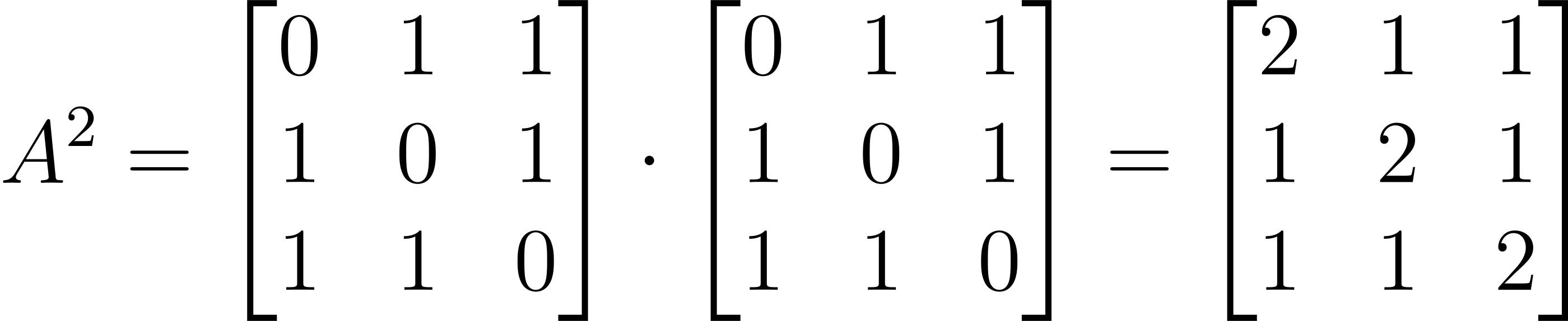
Each entry (i, j) gives the number of paths of length 2 from vertex i to vertex j.
For Example:
There are 2 paths of length 2 from vertex 1 to 1.
There is 1 path of length 2 from vertex 1 to 2.
And so on.
Question: Apply the transformation matrix to the vector.

Solution: