Measuring Welfare Using the Demand Supply Model
Course Progress and Roadmap
Review of Previous Topics: * Topic 1: Basics of the economic way of thinking. * Topic 2: How trade creates value. * Topics 3-5: The Demand-Supply Equilibrium framework as a tool to understand social issues. These topics were covered in Exam One.
Current Focus: Demand elasticity and its significance (recently completed).
New Objective (Day 7): Measuring welfare impacts. Specifically: * Consumer Surplus (CS): Measuring the well-being of buyers. * Producer Surplus (PS): Measuring the well-being of sellers. * Market Surplus: The sum of CS and PS to measure the overall well-being of all market participants.
The Utility of Welfare Measurement: * Example: A virus reduces the demand for pizza. While the demand-supply model predicts lower equilibrium prices and quantities, welfare tools evaluate whether these changes are "good" or "bad" for buyers, sellers, and society. * These measures allow for the illustration of how different policies impact market well-being through changes in surplus.
Learning Resources and Tasks
Khan Academy: Today’s lessons use videos from Sal Khan, who is noted for a manageable pace and detailed walkthroughs, contrasting with the faster pace of Jacob Clifford.
Task 1: Watch the videos (Consumer Surplus Parts A-C, Producer Surplus, Market Equilibrium/Welfare) and review notes.
Task 2: Take the Khan Academy Practice Quiz.
Task 3: Complete Homework 3 (the final portion of the lesson).
Consumer Surplus: Demand and Marginal Benefits
Conceptual Shift: Instead of viewing the demand curve as price driving quantity (), it is reconceptualized as quantity driving price ().
Marginal Benefit (MB): The demand curve represents the marginal benefit for each incremental unit. It defines the maximum "willingness to pay" (WTP) for that specific unit.
New Car Example (Discrete Units): * If only 1 car is sold per week, someone is willing to pay . This person’s MB is . * If 2 cars are sold, the second buyer might only be willing to pay (lower MB or a less excited buyer). * To sell 3 cars, the price must drop to the MB of the third buyer, which is . * To sell 4 units, the price must drop to the MB of the fourth unit, which is .
Defining Consumer Surplus (CS): * CS is the difference between what a consumer is willing to pay (marginal benefit) and what they actually pay (market price). * .
Calculating Total Consumer Surplus (Discrete Calculation): * If the price is set at to sell 4 units: * Unit 1: MB is . CS = . * Unit 2: MB is . CS = . * Unit 3: MB is . CS = . * Unit 4: MB is . CS = . This buyer is "on the fence." * Total CS: .
Calculating Consumer Surplus as an Area
The Area Method: For continuous markets (e.g., oranges), CS is the area below the demand curve and above the market price line.
Orange Stand Example: * Price () is set at per pound. * Quantity () sold is pounds. * The 100th pound has a marginal benefit of approximately . The buyer of this specific pound gets a surplus of . * To find the total CS for all 300 units, calculate the area of the triangle between the demand curve and the price line at . * Calculation: For a linear demand curve where the vertical distance (height) between the demand curve and the price line is and the base is units: * * CS = \frac{1}{2} \times 300\,\text{lbs} \times \2/\text{lb} = \
Calculus Note: If the demand curve is non-linear, thinner rectangles (integrals) are required for better approximations of the area.
Producer Surplus: Supply and Marginal Cost
Conceptual Shift: The supply curve is reconceptualized as an Opportunity Cost (or Marginal Cost) curve. It shows the minimum price producers must receive to be willing to produce that unit.
Resource Suitability: * The first units are produced using the "low-hanging fruit": the most suitable land, efficient labor, and best transportation networks. This results in a low marginal cost. * As quantity increases, producers must use less suitable land or less efficient labor, driving up the opportunity cost.
Berry Farm Example: * The first units have an average opportunity cost starting around per pound. * If the market price is , the producer sells the 4,000th unit exactly at its opportunity cost. * For the first units, the opportunity cost was lower than , creating a surplus for the producer.
Defining Producer Surplus (PS): * PS is the difference between the market price and the producer's marginal cost (opportunity cost). * .
Calculating Producer Surplus as an Area: * PS is the area above the supply curve and below the market price line. * In the berry farm example: Price = , Intercept (starting cost) = , Quantity = lbs. * * * PS = \frac{1}{2} \times \3/\text{lb} \times 4,000\,\text{lbs} = \ per week.
Market Equilibrium, Welfare, and Allocative Efficiency
Marginal Benefit (MB) vs. Marginal Cost (MC): * Market for Chocolate Example: The downward-sloping MB (Demand) curve represents the satiation of buyers. The upward-sloping MC (Supply) curve represents increasing production costs. * Surplus benefit is created whenever the marginal benefit of a unit is higher than its marginal cost ().
Allocative Efficiency: * This occurs at the quantity where . This is the equilibrium point in a perfectly functioning market. * At this quantity (), total market surplus (CS + PS) is maximized. * Units beyond this point () have an , meaning society incurs a net loss or negative surplus for those units.
Deadweight Loss (DWL): * Underproduction (): If the market produces less than the efficient quantity, potential surplus where is left "on the table." This lost surplus is called deadweight loss. * Overproduction (): If the market produces more than the efficient quantity, the cost of production exceeds the benefit. This net cost to society is also considered deadweight loss. * Ideally, a market produces the allocatively efficient quantity to avoid DWL in either direction.
Khan academy notes:
Lesson Overview: Consumer and Producer Surplus
This lesson introduced the basics of a branch of economics known as welfare economics, which is interested in how the allocation of resources affects wellbeing. The most important concepts used in welfare analysis are total surplus and allocative efficiency
The total surplus in a market is a measure of the total wellbeing of all participants in a market. It is the sum of consumer surplus and producer surplus.
Consumer surplus is the difference between willingness to pay for a good and the price that consumers actually pay for it. Each price along a demand curve also represents a consumer's marginal benefit of each unit of consumption. The difference between a consumer's marginal benefit for a unit of consumption, and what they actually pay, represents how much benefit a consumer get's from the price they are paying.
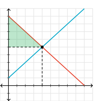
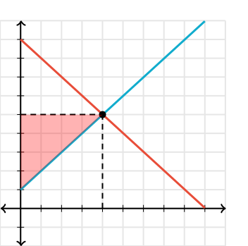
Producer surplus represents the difference between the price a seller receives and their willingness to sell for each quantity. Each price along a supply curve also represents a seller's marginal cost of producing each unit of production. Therefore the difference between what the price that the seller for each unit, and what it cost for the seller to produce that last unit, represents the seller's benefit from the price they are getting.
Total welfare is maximized when a market produces at its equilibrium price and quantity. This level of output is considered allocatively efficientbecause no other price and quantity combination can achieve a greater level of total surplus.

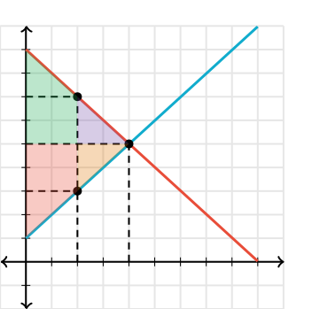

Total Surplus and Allocative Efficiency
Consumer and producer surplus together represent the total surplus, or total welfare in a market. Total welfare is the total extra benefit or happiness enjoyed by producers and consumers who feel they got a good price for the product being exchanged (paid less than they were willing to pay or received more than they were willing to accept).
The total welfare in a market is the combined areas of consumer surplus and producer surplus.
In the market for oranges above, the total welfare is the sum of the green and the red areas.
A market producing at equilibrium is achieving allocative efficiency, meaning that resource are allocated in the best possible manner to maximize total welfare among consumers and producers. Allocative efficiency is achieved when the price in the market equals the marginal benefit (\[MB\]) and the marginal cost (\[MC\]).
At any other price and quantity combination, the market would be allocatively inefficient, and the \[MB \neq MC\].
In the market above, the price and quantity supplied of oranges are lower than at equilibrium (\[\$3\] and \[2000\] pounds). The price consumers are willing to pay for the \[2000th\] pound of oranges (the \[MB\]) is greater than the cost of producing the \[2000th\] pound (the \[MC\]).
\[MB=\$7 > MC= \$3\].
The market is allocatively inefficient because consumers are willing to pay more than it costs producers to grow \[2000\] pounds of oranges. More resources should be allocated towards orange production.
The deadweight loss from the underproduction of oranges is represented by the purple (lost consumer surplus) and orange (lost producer surplus) areas on the graph.
In the market above the price and quantity supplied of oranges are greater than at equilibrium (\[\$7\] and \[6,000\] pounds). The price consumers are willing to pay for the \[6000th\] pound of oranges (the \[MB\]) is less than the cost of producing the \[6000th\] pound (the \[MC\])
\[MB = \$3 < MC = \$7\]
The market is allocatively inefficient because it costs producers more to produce \[6000\] pounds of oranges than consumers are willing to pay. Fewer resources should be allocated towards orange production.
The deadweight loss from the overproduction of oranges is represented by the purple (lost consumer surplus) and orange (lost producer surplus) areas on the graph.
Key terms
Term | Definition |
|---|---|
Consumer surplus | The welfare or benefit enjoyed by consumers who pay a price lower than the price they would have been willing to pay. Graphically the area below the demand curve and above the price in the market |
Producer surplus | The welfare or benefit enjoyed by producers who sell for a price higher than the price they would have been willing to sell for. Graphically the area above the supply curve and below the price in the market |
Total welfare (total surplus or community surplus) | The sum of consumer and producer surplus. Represents the total monetary benefit of consumers and producers who feel they got a good price for a product |
Allocative efficiency | When market output occurs at a quantity and price at which \[MB=MC\]. Neither too much nor too little is produced, and resources are allocated efficiently |
Allocative inefficiency | When a market is allocatively inefficient, the \[MB \neq MC\] at the prevailing price and quantity combination. Either too much or too little of the good is being produced |
Deadweight loss (DWL) | DWL is the loss of total welfare resulting from a market producing at an allocatively inefficient price and quantity combination |
Key calculation
Consumer and producer surplus can be calculated as areas on a demand and supply graph. The value used to describe total surplus is generally dollars, essentially quantifying the extra welfare in a market in terms of how much money consumers and producers feel like they have saved or earned through an exchange.
Consumer and producer surpluses are calculated as the areas of the triangles below \[D\] and above \[P_e\] (consumer surplus) and below \[Pe\] and above \[S\](producer surplus.
In the market above, consumer surplus can be determined by calculating the area of the green triangle:
\[\begin{aligned}CS &= \dfrac{1}{2} \times [(9-5) \times 4000]\\\\
&= \dfrac{1}{2} \times 16,000\\\\
&= \8,000\end{aligned}\]
Producer surplus can be determined by calculating the area of the red triangle.
\[\begin{aligned}PS&= \dfrac{1}{2} \times [(5-1) \times 4000]\\\\
&= \dfrac{1}{2} \times 16{,}000\\\\
&= \8{,}000\end{aligned}\]
Total welfare (total surplus) can be calculated by adding the sum of consumer surplus and producer surplus:
\[TW=\$8{,}000 + \$8{,}000 = \16{,}000\]
When a market is allocatively inefficient, the deadweight loss can be calculated.
The market above is inefficient because at the quantity of \[2,000\] oranges \[MB>MC\]. The welfare loss from the underproduction of oranges is represented by the purple and orange triangles, which can be calculated:
\[\begin{aligned}DWL&= \dfrac{1}{2} \times [(7-3) \times (4000-2000)]\\\\
&= \dfrac{1}{2} \times (4 \times 2000)\\\\
& = \4{,}000\end{aligned}\]
The loss of consumer and producer surplus from this market underproducing oranges equals \[\$4{,}000\].
Common errors and useful hints
The term surplus in the context of consumer, producer or community surplus should not be confused with the term surplus learned in earlier units. When the quantity supplied in a market exceeds the quantity demanded, we say there is a surplus in the market. This excess supply is undesirable and represents an overproduction of a good. Community surplus, on the other, is desirable and will be maximized when a market is achieving allocative efficiency.
Calculating areas of consumer and producer surplus or deadweight loss requires the ability to calculate the areas of both a triangle and a rectangle. Keep this equation in mind. For a triangle \[\text{Area} = \dfrac{1}{2} (\text{base} \times \text{height})\], and for a rectangle \[\text{Area} = \text{base} \times \text{height}\]