AP Microeconomics Unit 2 Notes

2.1 - Demand

2.2 - Supply

2.3 - Price Elasticity of Demand

2.4 - Price Elasticity of Supply

2.5 - Other Elasticities

2.6 - Market Equilibrium and Consumer and Producer Surplus

2.7 - Market Disequilibrium and Changes in Equilibrium

2.8 - The Effects of Government Intervention in Markets

2.9 - International Trade and Public Policy

Some info/photos taken from Jacob Clifford and ReviewEcon on youtube.

2.1 - Demand

When discussing demand, there is an assumption that there is a competitive market, meaning that multiple suppliers of a certain good/service exist and consumers can choose which to buy.

The Law of Demand

Demand - The different quantities of goods that consumers are willing and able to buy at different prices

Law of Demand - A law that states there is a negative relationship between the price of a good and the quantity demanded, ceteris paribus. (Microeconomics doesn’t cover exceptions to this rule, ignore them!)

• The Law of Demand states that as price increases, quantity demanded decreases, ceteris paribus.

• If the price is high, demand is low

• If the price is low, demand is high

• This can be visualized by auctions, the higher the price gets, the less bidders are there.

• Ceteris Paribus - Assuming all things remain the same; no other factor has changed.

The law of demand results from the income effect and submission effect

• Substitution Effect- When price increases, people are more likely to buy substitutes of a product because they are now relatively less expensive, so less units of the original good are sold

• Income Effect - People buy fewer units of goods when the price is high because they cannot afford it, and more when the price is low because they can afford it.

Demand Curve

The negative relationship between demand and price can be represented on a demand schedule (table) or demand curve. Something can move along the curve and the curve can be shifted. A change in price causes a change in quantity demanded, moving along the curve, while non-price Determinants of Demand, also known as shifters of demand, cause a change in demand and shift the entire curve. (more below)

Demand Schedule - A table showing how much of a food or service a consumer is willing and able to buy at different prices (ceteris paribus - all things equal) This data can be used to graph a demand curve

Demand Curve - A graph showing the data from the demand schedule which shows the relationship between demand and price.

A change in demand - A change in the demand at all prices, shifts the demand curve as the overall demand at all prices changes.

A change in quantity demanded - Following the law of demand, a supplier changes the price of a product along the demand curve, often due to lack of consumption. This does not shift the demand curve as the overall demand at all prices does not change, the price changes to a point of higher demand on the curve

Determinants (Shifters) of Demand - The 5 factors, not including price, that affect the demand of a product/service. Remember TRIBE

• Taste or Trends

  • ‘Trendy’ goods/services are in higher demand

• Related goods’ prices 

  • Substitutes: Prices of competitor goods/services.

    • If the price of cow milk increases, the demand for almond milk increases. If the price of cow milk decreases, the demand for almond milk decreases.

  • Complements: Price of items sold together, like gas and cars.

    • If gas prices go up, people are less likely to buy a large car, even though nothing about the car has changed.

• Income

  • How much money do consumers have to spend on a product?

  • The more money consumers have, the more money they will spend. The more money consumers have, the more likely high-end goods are to be sold.

• Buyers 

  • How many potential consumers are there?

• Expectations

  • If prices are expected to go up soon, the more people will consume. If the price is expected to go down, the less people will consume.

2.2 - Supply

Supply - The different quantities producers are willing and able to sell at different prices

The Law of Supply states as the quantity’s supplied increases, the price increases. A producer will charge more for more goods. Supply schedules (tables) and supply curves can represent the positive relationship between goods supplied and price, ceteris paribus. 

The Supply Curve

Determinants of the Curve (supply curve shifters) TIGERS

• Technology

  • New technology is invented to allow goods to be produced more efficiency 

• Input Costs

  • Cost of resources that the seller much consider

  • Labor costs

• Government

  • Taxes or incentives 

• Environmental shock or expectation

  • Is the price expected to go up soon? Sellers may sell less (or only for higher prices) to be able to sell with high profits, if they think the price is going to drop, they’ll try to sell quickly before the price drops.

  • Famine or sickness that makes it harder to produce a good, the good is more scarce and therefore more valuable.

• Related goods’ prices

  • What is the most money-making thing you can make with the resources you have?

  • If someone can make more money with the same resources producing a different product, they will, shifting the supply for the original product left, and the new product right

• Sellers

  • The more sellers, the market supply increases, so prices decrease.

Change in supply - change in the available supply regardless of a seller’s price, there is just less supply available. Shifts the supply curve.

Change in quantity supplied - A change in the quantity supplied at a certain price, the amount of supply the seller owns did not change, just the amount they will sell. Moves along the supply curve.

2.3 - Price Elasticity of Demand

Price Elasticity of Demand

Price Elasticity of Demand shows how responsive consumers are to price change. It is expressed as a graph or as a change in quantity demanded at a change to price.

Factors of Elasticity

• Substitutes

• Proportion of income

• Luxury vs necessity

• Addictiveness

• Time (need it in a hurry?)

Elastic Demand

• Goods with a lot of alternatives

• Luxuries

Inelastic Demand

• Goods with few/no alternatives

• Necessities

PED Coefficient/Equation

Remember NOOOO! and Queens are above princesses

• NO/O (New-old/old)

  • Percent change equations are all NO/O

• Queens over princesses (quantity/price)

For the answer/elasticity coefficient: Inelastic demand < 1 < elastic demand 

• PED > 1 - Elastic Demand

• PED < 1 - Inelastic Demand

• PED = 1 - Unit Elastic

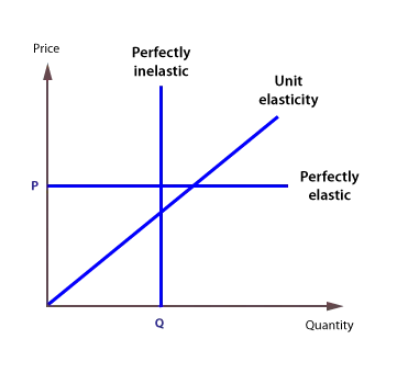
PED Curve

Elastic Demand - Flatter Curve

Perfectly Elastic Demand - Horizontal Curve

Inelastic Demand - Steeper Curve

Perfectly Inelastic Demand - Vertical Curve

2.4 - Price Elasticity of Supply

Price Elasticity of Supply (PES)

• Measures the responsiveness of quantity supplied with a change in price

• Shows if a good is elastic or inelastic

Determinates

• Length of time to make (more time = inelastic)

• Availability of inputs (easy to get = elastic)

• Ease of adjusting Factors of Production

PES Coefficient/Equation

Remember NOOOO and Queens are above princesses

• NO/O (New-old/old)

  • Percent change equations are all NO/O

• Queens over princesses (quantity/price)

For the answer/elasticity coefficient - Inelastic supply < 1 < elastic supply

• PES > 1 - elastic

• PES < 1 - inelastic 

• PES = 1 - Unit Elastic

PES Graph
Inelastic supply - Steeper

Elastic Supply - Flatter

Perfectly Inelastic - Vertical

Perfectly Inelastic - Horizontal

2.5 - Other Elasticities

Cross Price Elasticity of Demand (XED)

• Measures the responsiveness of quantity demanded for one product to a change of price in the other

• Shows if products are complements or substitutes

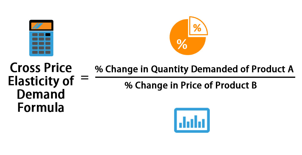
(Remember, percent change is always (N-O/O)

If… the goods are…

• XED is positive - substitutes 

• XED is negative - compliments 

Income Elasticity of Demand

Normal Good - A good that is purchased less when income decreases; most goods

Inferior Good - A good that increases as income decreases (ex: microwave meals, things more often purchased by those in a tight financial spot)

(Remember, percent change is always (N-O/O) If the coefficient answer is positive, it is a normal good. If the coefficient answer is negative, it is an inferior good.

• Positive - Normal Good

• Negative - Inferior Good

Total Revenue Test (Demand Only)

If Price ↑ and Total Revenue (TR) ↑, demand is relatively inelastic

If Price ↑ and TR ↓, demand is relatively elastic

If Price ↓ and TR ↑, demand is relatively elastic

If Price ↓ and TR ↓, demand is relatively inelastic

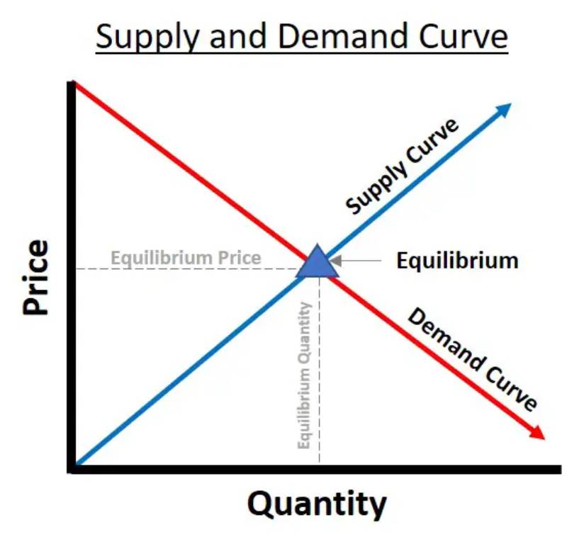
2.6 - Market Equilibrium and Consumer and Producer Surplus

Market Equilibrium is the point where the supply curve and the demand curve meet. Always assume a market is at equilibrium unless stated otherwise, because over time, free markets will always return to the equilibrium point If the price is too high, there will be a surplus of goods, so sellers will lower the price so they sell, returning to equilibrium. If the price is too low, there will be a shortage, and sellers will increase their price to make more money, returning to equilibrium

Consumer surplus - the difference between what consumers are willing to pay vs what theyre actually paying (the equilibrium price)

• If a consumer is willing to spent 5$ on a good, but the equilibrium price means that the good is only being sold for 3$, that extra 2$ is the consumer’s surplus.**

Producer Surplus - the difference between what producers are willing to sell their goods for, vs what they’re actually selling their goods for (the equilibrium price)

• If a producer is wiling to sell their produce for 7$, but the equilibrium price means they are able to sell their good at 10$, the extra 3$ is there surplus.**

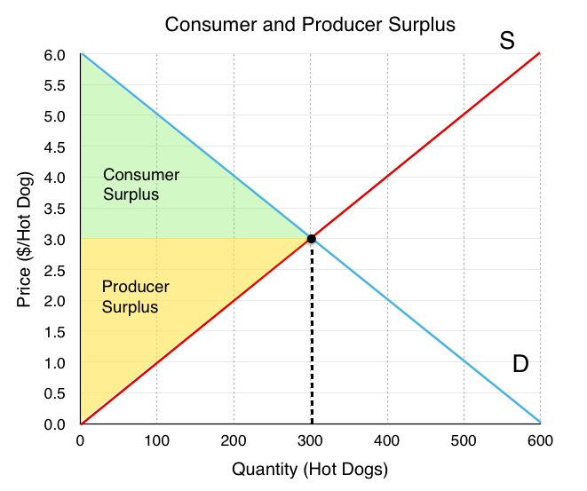
**However, calculating the total consumer or producer surplus is more complicated. It is calculated using the formula for the area of a triangle, A = (1/2)BH (B=base H=height).

• In the graph above, the consumer surplus is (1/2)(300)(3) = 450

• In the graph above, the producer surplus is (1/2)(300)(3) = 450

• The consumer and producer surplus will always be equal at equilibrium.

2.7 - Market Disequilibrium and Changes in Equilibrium

Whenever a market is not at equilibrium, it is an inefficient market. In inefficient markets, there is deadweight loss (DWL) DWL decreases the consumer and producer surplus

In this graph, the price is put at P2, and red shows the deadweight loss.

When the demand or supply curve shifts, the equilibrium point changes. On the AP Tets, you will likely need to determine the equilibrium price on a supply/demand graph, how a change will impact the supply and demand curves, find the new equilibrium price/quantity, and compare it to the original.

• In this example, there is a new Tax shifting the supply curve left/up

• There is now DWL

• The new equilibrium price, Pb, is greater than the original, Pe

• The new equilibrium quantity, Qt is less than the original, Qe

When both demand and supply shift, either the price or the quantity will become indeterminate

• In the graph below, price appears to not change, but depending on how you draw the graph (how far you shift each curve), that will change, making it indeterminate. The change in price may change depending on how much you move the curves, which is why it is indeterminate, but quantity will always increase.

• The second graph shows how, with the same shifts, the price will appear lower, because price is indeterminate.

2.8 - The Effects of Government Intervention in Markets

The government may intervene in free markets:

• To ensure equity (ex:make sure people can afford their medication)

• As a result of to political pressure (lobbying, corruption)

• To promote a certain agenda

There are two kinds of price controls 

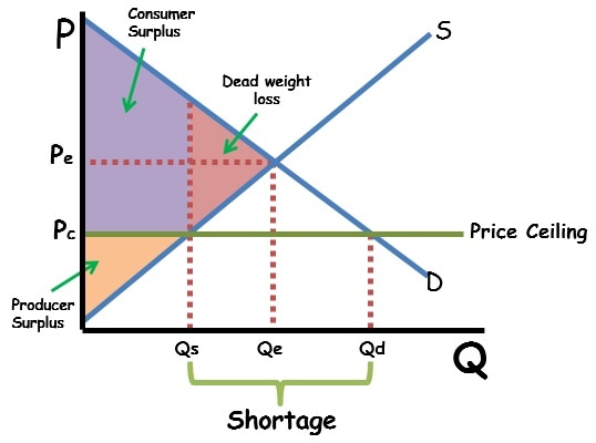
• Price ceiling/cap

  • A maximum price sellers can charge for a good

  • Only effective if put below the current market equilibrium

    • If not, its a non-binding price ceiling

  • Creates a shortage of goods

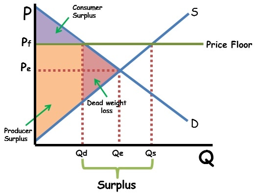
• Price floor

  • The minimum price a seller can charge for a good

  • Only effective if put above the current market equilibrium

    • If not, its a non-binding price floor

  • Creates a surplus, which the government generally must buy up the shortage (ex: the cheese caves. google it, its fun)

  • May be done to support farmers, protect fair wages 

Price Ceiling

Price Floor

Potential consequences of price caps

• Wasted resources - rationing causes people to have to wait in lines for get the good, looses opportunity costs

• Inefficient allocation - people who need/want the good can’t get it

• Inefficiently low quantity - Seller can’t afford to improve the product. (Ex, rent so cheap repairs can’t be made)

• Black markets - dangerous and government loses tax revenue

Potential consequences of price floors

• Inefficient allocation - sales at a lower price cannot occur

• wasted resources - the government must buy the surplus, a company may have to fire people as they have to pay them more so people are left jobless

• Inefficiently high quantity - if the government will always buy the product, there is no incentive to improve. 

• Black market - Paying people under the table, government loses tax money

2.9 - International Trade and Public Policy

Public Policy - The rules and regulations that govern international trade

Quota - A government-imposed maximum of goods that can be imported. Protects/encourages domestic manufacturing

• Quota graphs are NOT on the AP Exam

Tariff - A tax on foreign-made goods. The price is often shared by producers and consumers. Protects/encourages domestic manufacturing

This graph shows the domestic supply and demand curve, and the World Price for the same good.

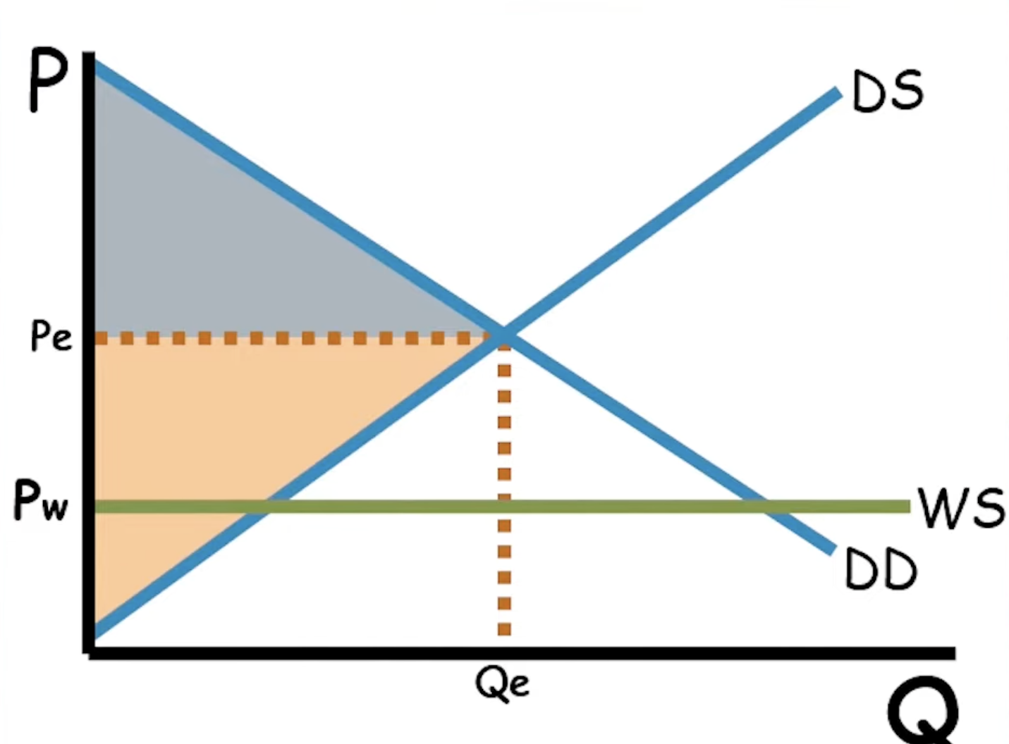
If this country opens itself up to world trade, the price will lower to the world price, causing domestic sellers to only produce at Qs, but consumers will demand at Qd. The difference will be supplied by foreign producers.

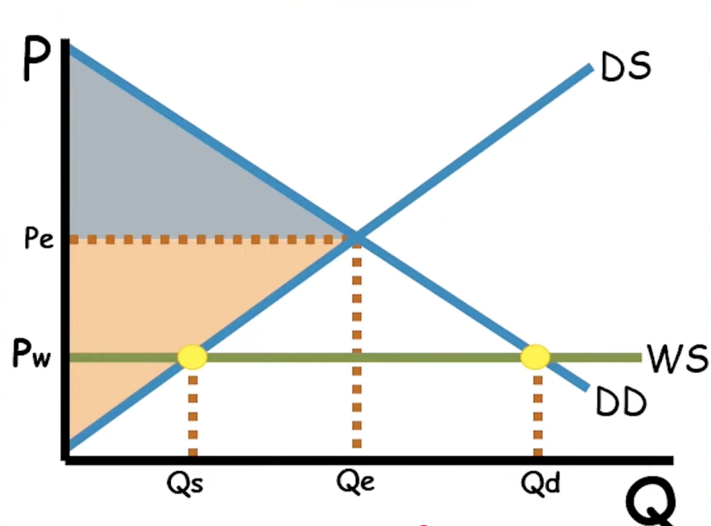
This significantly increases the consumer surplus (gray), but reduces the producer surplus (orange)

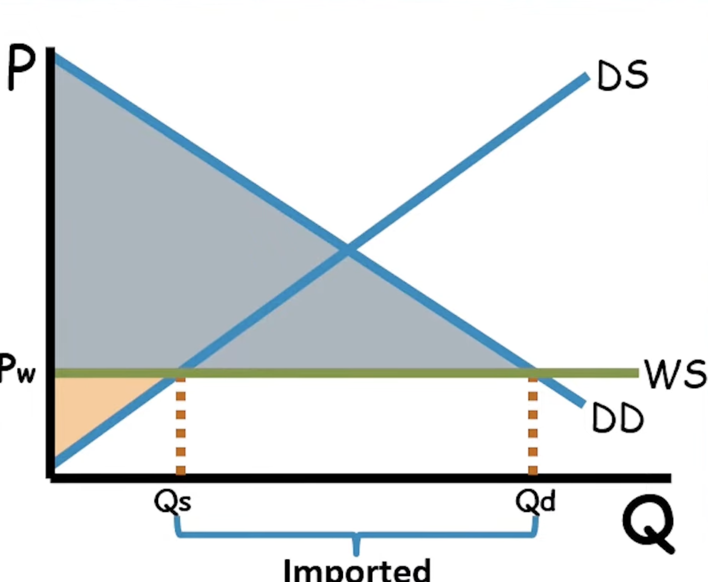
In short, if the world price is below equilibrium

• Consumers will demand more

• Domestic suppliers will produce less

• The difference will be imported

• There is more consumer surplus

• There is less producer surplus

• increase total economic surplus

In contrast, if the world price is above market equilibrium, consumers will demand less, and suppliers will produce more, and export all that isnt bought by domestic consumers (the different).

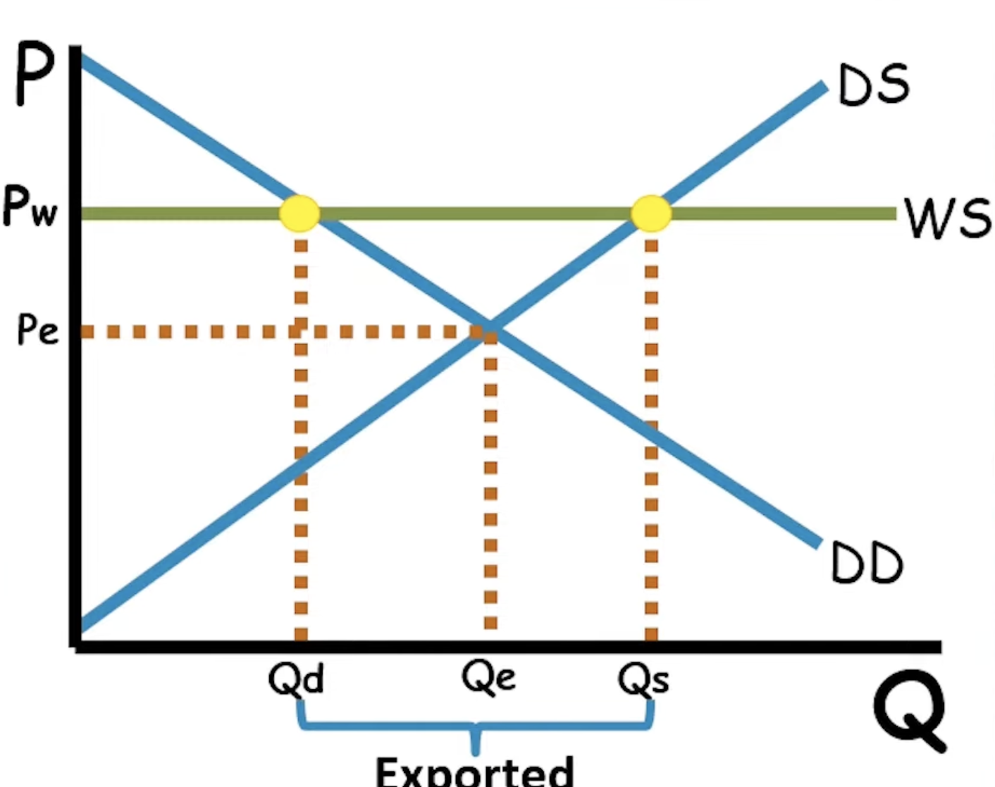
Consumer surplus decreases, and producer surplus increases

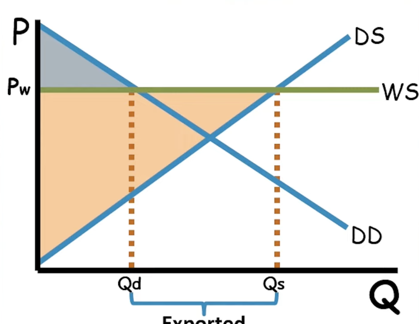
In short, if the world price is above equilibrium

• Consumers will demand less

• Domestic suppliers will produce more

• The difference will be exported

• There is less consumer surplus

• There is more producer surplus

• increase total economic surplus

Tariffs

If a tariff is imposed, the world price will be higher. Quantity supplied and demanded move along their respective curves to meet the new WS. Qs → Qs1 and Qd → Qd1

Producer surplus will increase, Consumer surplus will decrease, there will be dead-weight loss, and tariff revenue for the government.

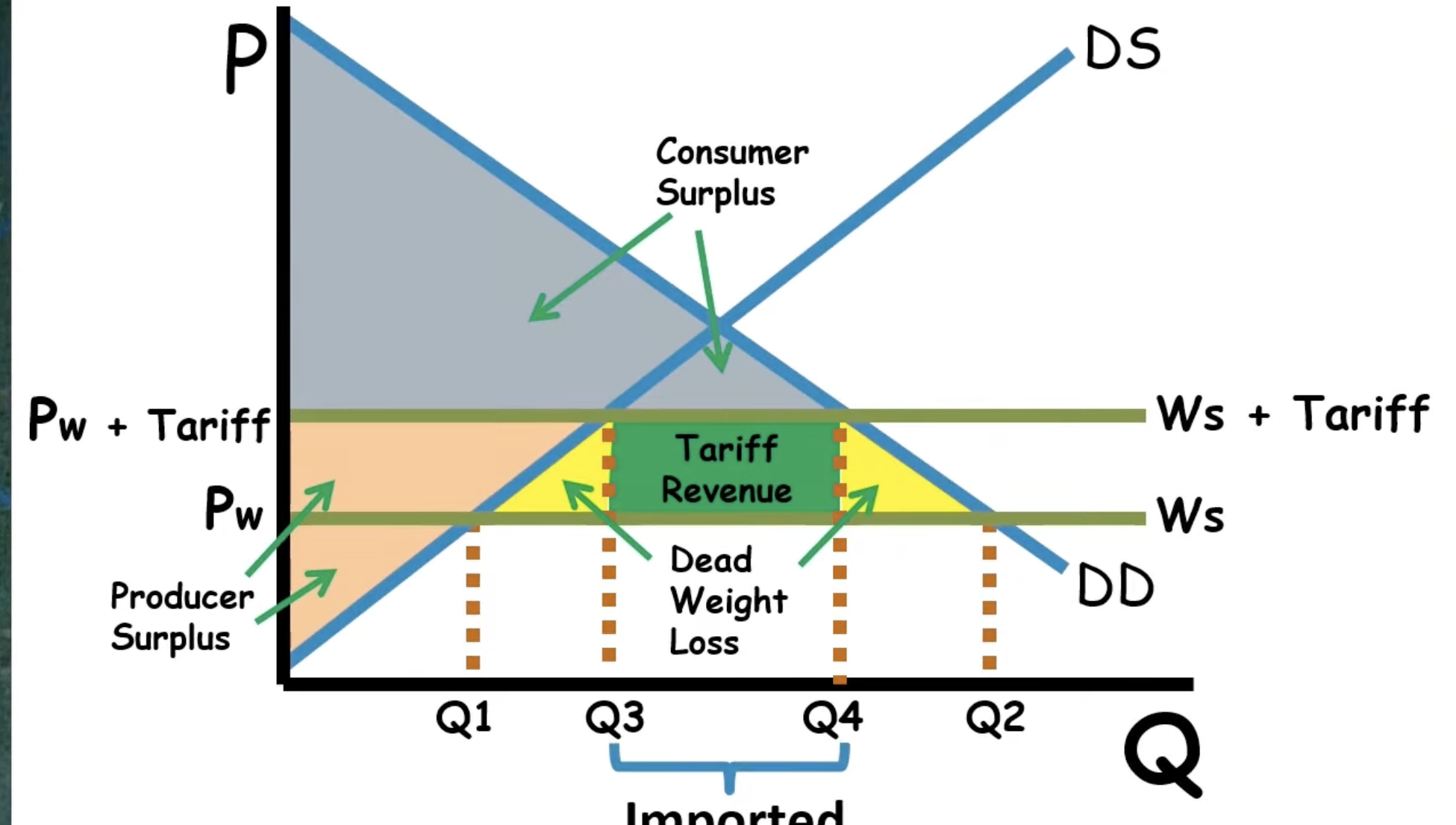
Tariffs

• Decrease trade

• Decrease total economic surplus

• Create DWL