Statistics and probability (IB)
Descriptive Statistics
Population and Sample
In statistics, when we talk about a population, we mean every single person or thing we're interested in studying. Think of it as the whole pie. A sample, on the other hand, is just a slice of that pie – a smaller group taken from the population to represent the whole. For instance, if we want to know about the heights of all students in a school (the population), we might measure just 100 students picked randomly (the sample) to get an idea.
Random Sampling
To put it simply, a random sample is like picking names out of a hat where everyone in the group has the same chance of getting their name drawn. This fairness is really important because it helps make sure that the small group we pick actually reflects the bigger group we're interested in.
Data Types
Data comes in two main types: discrete and continuous.
Discrete data is like counting whole things – it can only be certain separate values, usually whole numbers. Think of it as things you can count, like the number of students in a class.
Continuous data, however, is like measuring things – it can be any value within a range. Imagine the height of students; it could be any value within a certain span, not just whole numbers.
Reliability and Bias
In statistics, it's really important to think about how trustworthy your information is (reliability) and if your sample is fair (bias). If your sample doesn't truly reflect the whole group you're studying, that's called bias, and it can mess up your results.
Outliers
In statistical analysis, outliers are defined as observations that deviate markedly from the predominant pattern of the dataset. These anomalous data points, being significantly disparate from the central cluster of values, possess the potential to exert a disproportionate influence on statistical outcomes and therefore warrant meticulous evaluation.
Data Presentation
Frequency Distributions
A frequency distribution is a tabulation or graphical representation that organizes observed data to illustrate the incidence of each distinct value within a dataset. This method effectively summarizes the dataset by displaying the count of occurrences for every unique value, thereby revealing the underlying pattern of data dispersion.
Histogram
In statistical representation, histograms function as bar graphs specifically designed to depict the frequency distribution of continuous data. In a histogram, the horizontal axis (x-axis) is scaled to represent the range of data values, typically grouped into contiguous intervals or bins, while the vertical axis (y-axis) quantifies the frequency, or count, of observations falling within each respective interval.
Cumulative Frequency Graphs
also known as ogives, are graphical tools that illustrate the accumulated frequency of data values up to and including each interval. These representations are particularly valuable in statistical analysis as they facilitate the determination of key positional measures, such as the median and percentiles, directly from the visual depiction of the data's distribution.
Box and Whisker Diagrams
commonly referred to as box plots, are graphical instruments employed to furnish a concise visual synopsis of a dataset's distribution. These diagrams effectively represent key statistical measures including the median, quartiles, and the identification of potential outliers within the data.
Measures of Central Tendency and Dispersion
Central Tendency
Mean: This is the arithmetic average, calculated as the sum of all values in a dataset divided by the total number of values.
Median: Representing the central value in a dataset, the median is identified as the midpoint of the ordered data, dividing the distribution into two equal halves.
Mode: The mode denotes the value that appears with the highest frequency within the dataset, indicating the most typical or common observation.
Dispersion
Range: Defined as the extent of data spread, the range is calculated by subtracting the minimum value from the maximum value in the dataset.
Variance: This measure quantifies the average of the squared differences of each data point from the mean of the dataset. It provides an indication of the overall dispersion around the mean.
Standard Deviation: Representing the square root of the variance, the standard deviation is a widely used measure of dispersion. It expresses the degree of data spread in the original units of measurement, offering a more interpretable measure of variability.
Linear Correlation and Regression
Correlation
Correlation, in statistical terms, is a measure that quantifies both the intensity and the direction of the linear association between two paired variables. This relationship is encapsulated by the correlation coefficient, denoted as r, which is dimensionless and scaled to range from -1 to +1.
The interpretation of the correlation coefficient r is as follows:
A value of r = +1 signifies a perfect positive correlation, indicating that as one variable increases, the other variable increases proportionally in a perfectly linear manner.
Conversely, a value of r = -1 represents a perfect negative correlation, denoting a perfectly linear inverse relationship where an increase in one variable is accompanied by a proportional decrease in the other.
A correlation coefficient of r = 0 suggests no linear correlation between the two variables, implying the absence of a linear trend in their relationship, although it does not preclude the possibility of a non-linear association.
Regression
Linear regression is a statistical method used to model the linear relationship between two variables by determining the optimal straight line that best fits a given set of data points. This line is mathematically represented by the equation y = mx + c, where:
y represents the dependent variable.
x represents the independent variable.
m denotes the slope of the line, indicating the rate of change in y for a unit change in x.
c signifies the y-intercept, representing the value of y when x is zero.
Probability
Basic concepts
Trial: A trial constitutes a singular performance or instance of a defined experiment.
Outcome: An outcome is defined as a specific, observable result that may arise from the execution of a trial.
Probability: Probability is a numerical quantification of the likelihood of a particular event's occurrence. It is expressed as a value on a scale from 0 to 1, inclusive, where 0 indicates impossibility and 1 indicates certainty
Probability Calculations
Venn diagrams: These diagrams are primarily employed to visualize and calculate probabilities associated with set operations. They are particularly useful for problems involving the union, intersection, and complement of events, allowing for a graphical representation of relationships between events and their probabilities.
Tree diagrams: Tree diagrams are specifically designed for analyzing sequential events, where the outcome of one event influences subsequent events. By branching out to represent each possible outcome at each stage, these diagrams facilitate the calculation of probabilities for compound events occurring in sequence.
Sample space diagrams: These diagrams serve as a systematic method for enumerating and visualizing all potential outcomes of an experiment. By mapping out the entire sample space, they provide a comprehensive framework for determining probabilities, particularly in scenarios with a limited number of possible outcomes.
Conditional Probability
Conditional probability refers to the measure of the likelihood of an event, denoted as event A, occurring, given that another event, denoted as event B, has already taken place. This probability is symbolized as P(A|B), which is verbally expressed as "the probability of A given B".
Mathematically, conditional probability is defined by the formula:
P(A|B) = P(A ∩ B) / P(B)
where:
P(A|B) is the conditional probability of event A occurring given that event B has occurred.
P(A ∩ B) is the joint probability of both event A and event B occurring.
P(B) is the marginal probability of event B occurring.
Discrete Random Variables and Probability Distributions
A discrete random variable is defined as a variable whose possible values are confined to a countable set. This implies that the variable can only assume specific, distinct values, often integers, with no intermediate values permissible within its range.
Associated with each discrete random variable is a probability distribution. This distribution mathematically delineates the likelihood of the random variable assuming each of its possible values. In essence, it provides a comprehensive mapping of all potential outcomes of the variable and their corresponding probabilities.
Expected Value
The expected value, denoted as E(X), of a discrete random variable X represents the theoretical average value of X over a large number of repeated trials. It is calculated as the summation of the product of each possible value (xᵢ) that the random variable can assume and its corresponding probability (P(X=xᵢ)). The formula, E(X) = ∑xᵢP(X=xᵢ), essentially weights each potential outcome by its likelihood of occurrence, providing a measure of the variable's central tendency in a probabilistic sense.
𝐸(𝑋)=∑𝑥𝑖𝑃(𝑋=𝑥𝑖)
Binomial Distribution
The binomial distribution is a discrete probability distribution that mathematically describes the number of successful outcomes in a predetermined number of independent Bernoulli trials. Each trial is characterized by an identical and constant probability of success.
If X ~ B(n, p), where n is the number of trials and p is the probability of success on each trial:
𝑃(𝑋=𝑘)=(𝑛𝑘)𝑝𝑘(1−𝑝)𝑛−𝑘
Normal Distribution
The normal distribution is a fundamental continuous probability distribution characterized by a symmetric, bell-shaped curve. This distribution is uniquely defined by two parameters: its mean (μ), which dictates the central location of the curve, and its standard deviation (σ), which governs the spread or dispersion of the distribution around the mean.
Standard Normal Distribution
The standard normal distribution is a specific instance of the normal distribution distinguished by a mean (μ) of zero and a standard deviation (σ) of unity. This particular form serves as a foundational reference within statistical analysis due to its simplified parameters.
To facilitate comparisons and calculations across diverse normal distributions, any normally distributed variable can be transformed into a standard normal variable through a process of standardization. This transformation is achieved using the z-score, which is calculated as follows:
z = (x - μ) / σ
where:
z represents the standardized value, or z-score.
x is the raw score or observed value from the original normal distribution.
μ is the mean of the original normal distribution.
σ is the standard deviation of the original normal distribution.
The z-score essentially quantifies the number of standard deviations that a particular raw score x is away from the mean μ of its distribution. This standardization process enables the use of standard normal distribution tables or computational tools to determine probabilities associated with any normal distribution, regardless of its original mean and standard deviation.
Normal Probability Calculations
To determine probabilities associated with normal distributions, the standard procedure involves a two-step process:
Standardization: Initially, the raw value of interest is transformed into a z-score. This is accomplished through the application of the z-score formula, which effectively converts the value from its original normal distribution to its corresponding position within the standard normal distribution.
Probability Determination: Subsequently, the calculated z-score is utilized to ascertain the desired probability. This step typically entails consulting standard normal distribution tables or employing computational technology capable of evaluating cumulative probabilities for the standard normal distribution. These resources provide the area under the standard normal curve, which directly corresponds to the probability of observing a value less than or greater than the standardized value, or within a specified range of standardized values.
Bayes’ Theorem
Bayes' Theorem establishes a mathematical relationship between conditional probabilities, specifically articulating how to revise the probability of an event based on new evidence. The theorem is formally expressed as:
P(A|B) = [P(B|A) * P(A)] / P(B)
Continuous Random Variables and Probability Density Functions
In dealing with continuous random variables, we shift from using probability mass functions to probability density functions (PDFs). Unlike discrete variables where we can talk about the probability of a variable exactly equaling a specific value, for continuous variables, the chance of hitting any single, precise number is essentially zero. Instead, PDFs describe the relative likelihood of the variable taking on a value near a given point. To find the probability that a continuous variable falls within a range of values, we need to calculate the area under the PDF curve over that range, which is done using integration.
Properties of Continuous Distributions
For a continuous random variable X with PDF f(x):
Mode: The value of x where f(x) is maximum
Median:

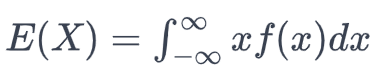
Mean:
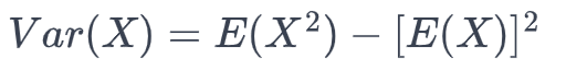
Variance:
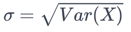
Standard Deviation:
Linear Transformations
In the realm of linear transformations of random variables, if we define a new random variable Y as a linear function of another random variable X, such that Y = aX + b, where a and b are constants, then the statistical properties of Y, specifically its expected value and variance, are directly related to those of X through the following established relationships:
Expected Value of Y: The expected value of Y, denoted as E(Y), is given by the linear transformation of the expected value of X. This is expressed as:
E(Y) = aE(X) + b
This formula indicates that the expected value of the transformed variable Y is obtained by multiplying the expected value of X by the constant a and subsequently adding the constant b. In essence, linear transformations are preserved under the expectation operator.
Variance of Y: The variance of Y, denoted as Var(Y), is related to the variance of X by the square of the constant multiplier a. This relationship is formalized as:
Var(Y) = a²Var(X)