Ch2 Probability Concepts and Applications (1)
Title: Data & Decision Analysis
Focus: Chapter 2 - Probability Concepts and Applications
Instructor: Dr. Yuanxiang John Li
Page 2
Chapter Outline:
Fundamental Concepts
Revising Probabilities with Bayes’ Theorem
Further Probability Revisions
Random Variables
Probability Distributions
The Binomial Distribution
The Normal Distribution
The F Distribution
The Exponential Distribution
The Poisson Distribution
Introduction:
Life is uncertain; predicting future events is typically challenging.
Probability: A numerical representation of the likelihood that an event will take place.
Two Basic Rules of Probability:
The probability of an event is always between 0 and 1, where 0 indicates impossibility and 1 indicates certainty.
The sum of the probabilities of all possible outcomes of a random experiment must equal 1.
Probability P(event) ranges from 0 to 1: 0 ≤ P(event) ≤ 1
P = 0 indicates impossibility; P = 1 indicates certainty.
The sum of probabilities of all possible outcomes equals 1.
In addition, the probability of the complement of an event can be calculated as P(not event) = 1 - P(event), which helps in determining the likelihood of an event not occurring.
Types of Probability:
Objective Approach: Based on relative frequency of events.
Subjective Approach: Involves personal judgment; used in areas like opinion polls and expert consultations (Delphi method).
Page 6
Objective Probability can be calculated using classical or logical methods, e.g., through trials to observe outcomes and establish probabilities.
Relative Frequency Approach:
Diversely Paint Example: Historical painting demand observed over 200 days.
Probability Calculations:
0 gallons: P(0) = 0.20
1 gallon: P(1) = 0.40
2 gallons: P(2) = 0.25
3 gallons: P(3) = 0.10
4 gallons: P(4) = 0.05
Total probabilities sum to 1.
Definition of Experiment and Event:
An experiment has well-defined possible outcomes (sample space).
An event is a subset of outcomes to which a probability is assigned.
Mutually Exclusive Events:
Events that cannot occur simultaneously; e.g., outcomes of a coin toss (heads or tails).
Venn Diagrams:
Used to illustrate mutually exclusive and non-mutually exclusive events.
Collectively Exhaustive Events:
A complete set of outcomes covering all possibilities.
Examples: Outcomes of a die roll; coin flips (heads and tails).
Card Drawing Example:
A = event of drawing a 7; B = event of drawing a heart.
Ask about mutual exclusiveness and collective exhaustiveness.
More on Card Drawing Example:
P(7) = 4/52 and P(heart) = 13/52.
Events A and B are not mutually exclusive (7 of hearts exists).
Mutually Exclusive & Collectively Exhaustive:
Examples of events in a card draw scenario and whether they fit into these classifications.
Intersections of Events:
The intersection A ∩ B: common outcomes of both events.
Joint Probability notation: P(A ∩ B).
Unions of Events:
The union A ∪ B: outcomes in either A or B.
Additive rule: P(A ∪ B) = P(A) + P(B) - P(A ∩ B).
Example Intersection/Union:
Calculate P(A ∩ B) and P(A ∪ B) from previous card example.
Calculating Probabilities:
P(A ∩ B) = 1/52; P(A ∪ B) = 16/52.
The Additive Rule:
Total probability for A or B calculated through the additive rule explained.
Conditional Probability:
Probability that one event occurs given that another event has already occurred.
Independent Events:
If event A does not affect event B, they are independent.
Example scenarios to illustrate independence.
Independent Events Example:
Fair coin toss illustrating independence of two draws.
Example with Balls:
Probability calculations for drawing black and green balls from a bucket.
Continuation of Balls Example:
Probabilities remain same due to replacement in drawing process.
Brief Summary:
Key concepts highlighted: complement events, mutually exclusive vs independent events.
Random Variables:
Definition and types: discrete (limited values) vs continuous (infinite values).
Examples of Random Variables:
Questionnaire responses and item inspections illustrate discrete variables.
Construction completion percentage relates to continuous variables.
Discrete Probability Distribution:
Assigning probabilities to outcomes in discrete settings. Example: class quiz scores.
Discrete Probability Distribution Continued:
Mean (expected value) and variance discussed.
Expected Value:
Defined and illustrated through quiz score example.
Variance Calculation:
Explains variance and its calculation through quiz example.
Standard Deviation:
Connection to variance; calculation example shown.
Excel and Probability Distributions:
Tools demonstrated for managing discrete probability in an Excel framework.
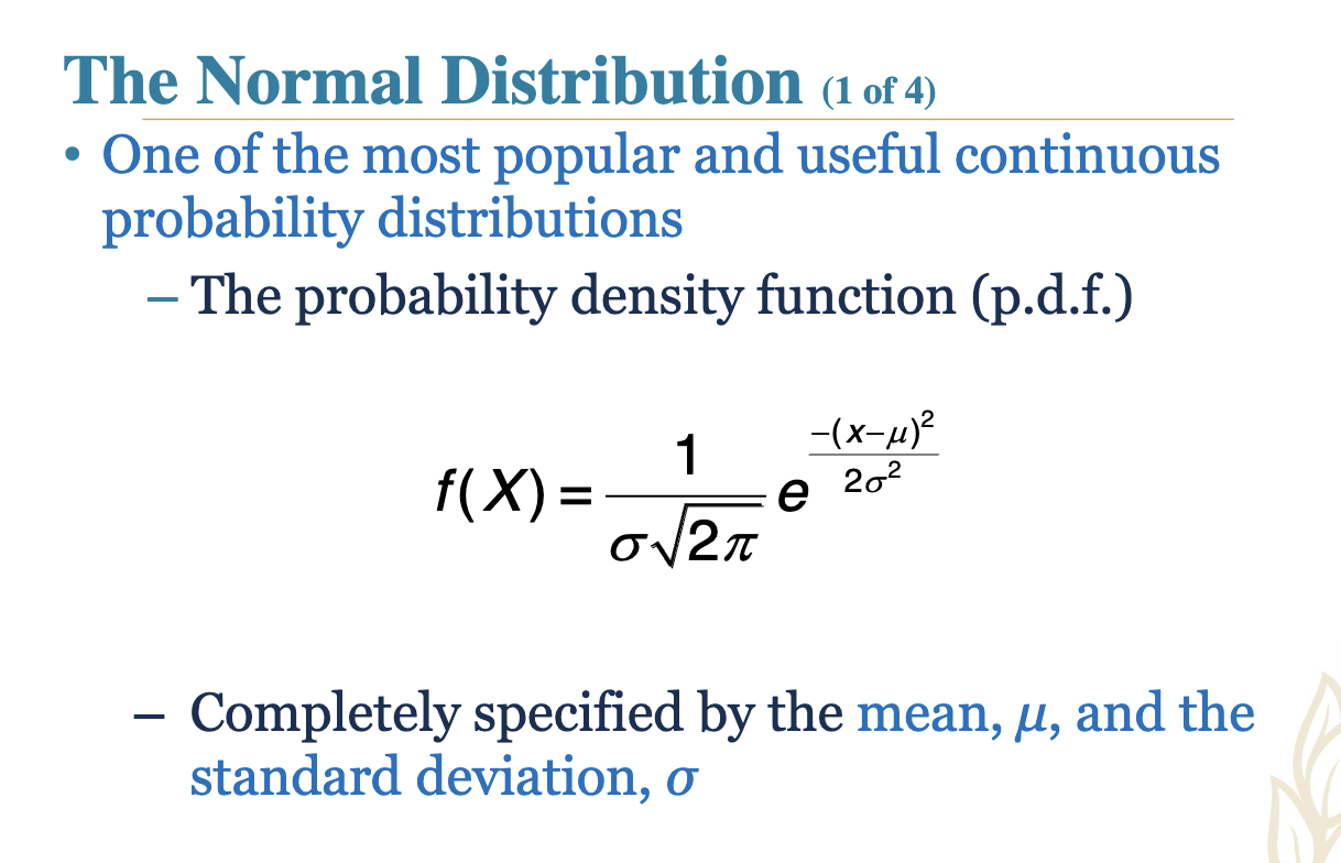
Continuous Random Variables
Defined by probability density functions.
Characteristics outlined.
Probabilities in continuous distributions explained.
Comparison of Discrete vs Continuous Distributions
Discrete
• Variable can only take on certain values
• Probabilities can be assigned to the values in the distribution
• Binomial Distribution
• Poisson Distribution
Continuous
• Variable can take on any value within a specified range (which may be infinite)
• Has an infinite number of possible values
• Probability associated with any particular value of a continuous distribution is null
• Normal Distribution
• F Distribution
• Exponential Distribution
Bernoulli Process
Many business experiments can be characterized by the Bernoulli process
• The Bernoulli process is described by the binomial probability distribution
1. Each trial has only two possible outcomes
2. The probability of each outcome stays the same from one trial to the next
3. The trials are statistically independent
4. The number of trials is a positive integer
Binomial Distribution
The binomial distribution is used to find the probability of a specific number of successes in n trials
Solving Problems with the Binomial Formula
Example: Probability obtained from coin toss outcomes.
P(r successes in n trails)
where
– n = number of trials
– r = number of successes
– p = the probability of success on any single trial
– q = 1 − p = the probability of a failure
• The symbol “!” means factorial:
– n! = n(n − 1)(n − 2)...(1). For example, 4! = 4*3*2*1= 24
– By definition: 1! = 1 and 0! = 1!
!( )!
r n rn p q
r n r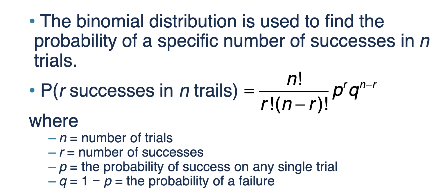
MSA Electronics Example
Probability problem related to defective transistors set within binomial distribution context.
Using Binomial Tables
Displaying binomial probabilities through reference tables.
Binomial Distribution Expected Values
Explanation in relation to experiments.
Excel Functions for Binomial Distribution
Highlighting practical Excel formulas for calculating binomial probabilities.
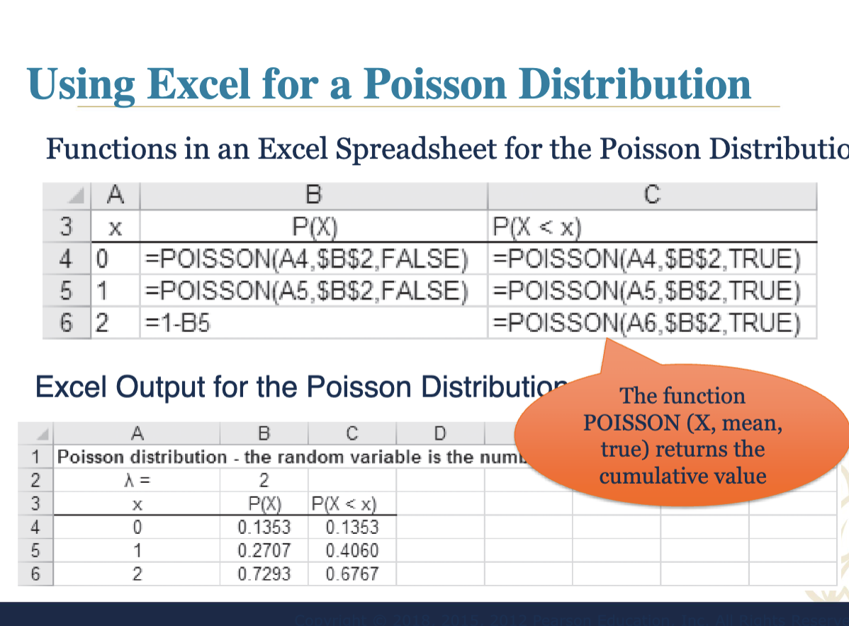
Poisson Distribution
Description and application in scenarios involving arrival rates.
The Poisson Distribution (1 of 3)
• A discrete probability distribution
– Often used in queuing models to describe
arrival rates over time or describe the number
of random arrivals per some time interval
– Poisson does not have a given number of trials
(n) as a binomial experiment does
– Occurrences are independent one another
– Occurrences occur over an interval
– e.g., the number of random customer arrivals
per five-minute interval at a small boutique on
weekday mornings
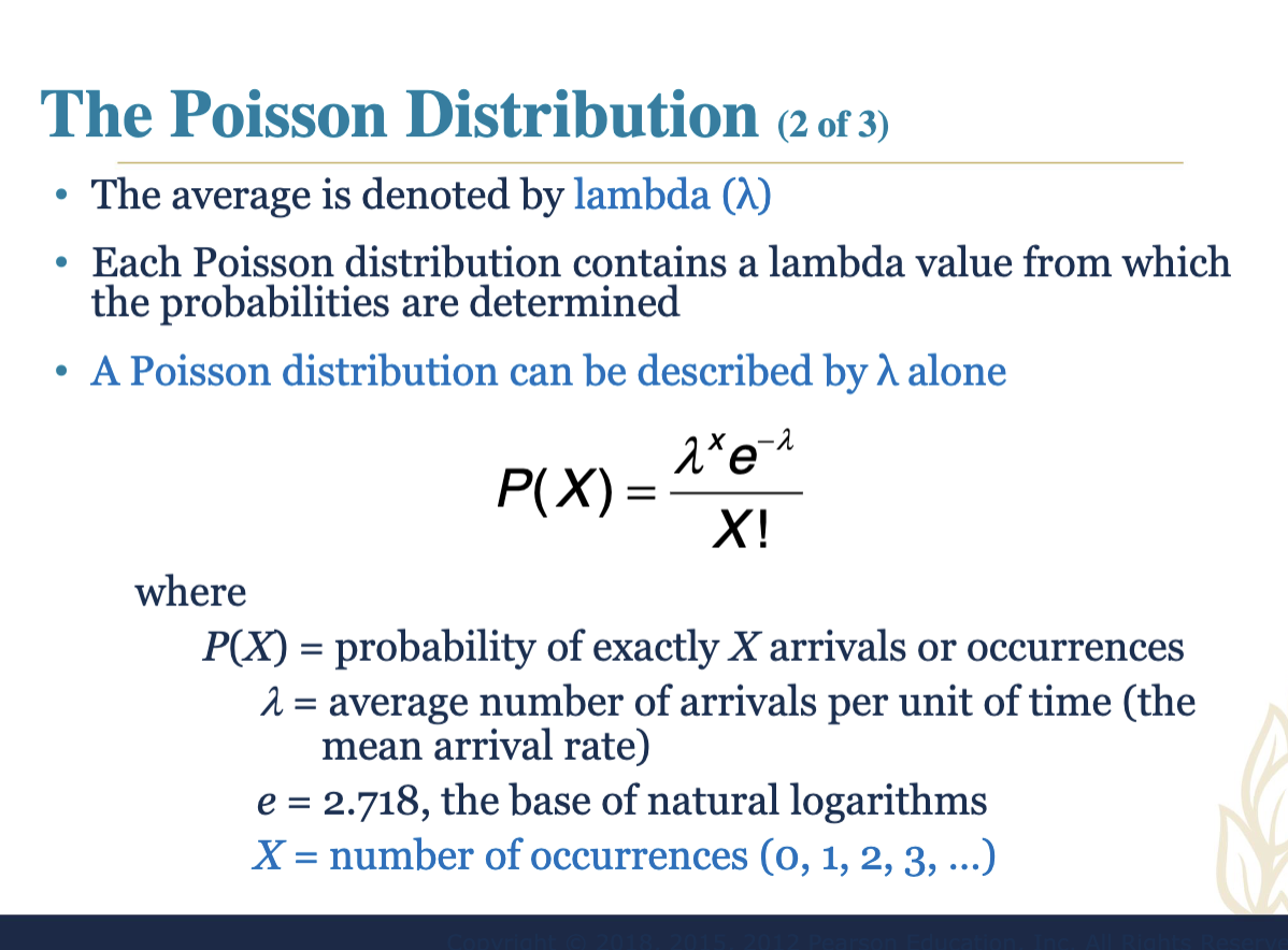
Poisson Distribution Average
Definition of Lambda (λ); the average
Sample Poisson Distribution Graphs
Display of sample graphs for understanding Poisson distribution behavior.
Sample Poisson Distribution graphs displayed.
These graphs illustrate how the distribution varies with different values of λ, showcasing the probability of a given number of events occurring in a fixed interval.
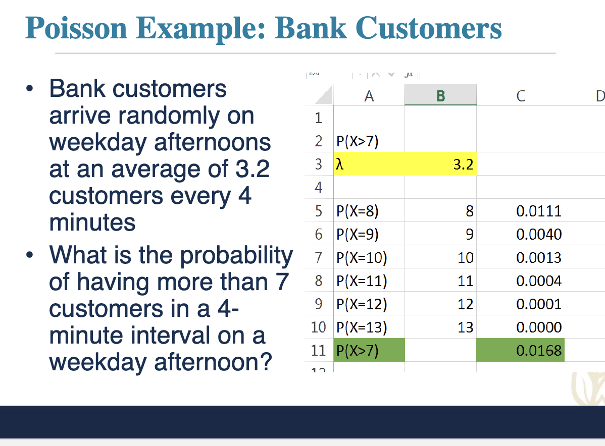
Bank Customers Example:
Estimation of customer arrivals applied through Poisson distribution.
Page 51
Expected Value & Variance in Poisson Distribution:
Calculated with bank customers example.
Poisson: Expected Value & Variance
• A Poisson Distribution:
Expected value (mean) = λ
Variance = λ
• For the Bank Customers example
Expected value = 3.2
Variance = 3.2
Normal Distribution:
Overview and significance in statistics.
Normal Distribution with Different Values for μ
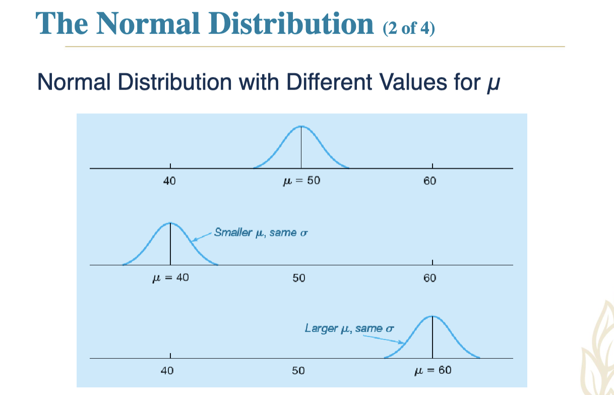
Visual representation of Normal Distribution variations based on standard deviation adjustments.
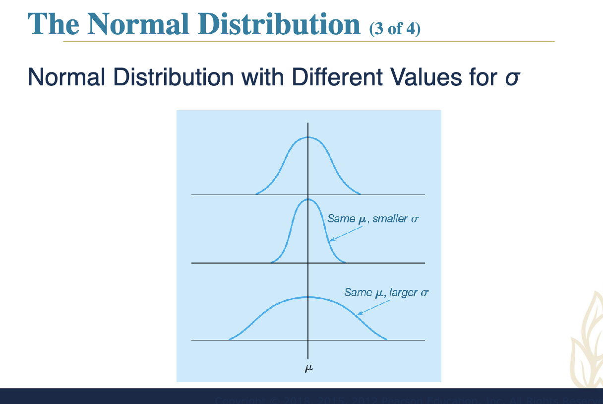
Characteristics of Normal Distribution explained visually.
Symmetrical with the midpoint representing the mean
Shifting the mean does not change the shape
Values on the X axis measured in the number of standard deviations away from the mean
As standard deviation becomes larger, curve
flattensAs standard deviation becomes smaller, curve
becomes steeper
Standard Normal Distribution:
Step 1
• Convert the normal distribution into a standard normal
distribution
– Mean of 0 and a standard deviation of 1
– The new standard random variable is Z= X- μ /σ
where
X = value of the random variable we want to measure
μ = mean of the distribution
σ = standard deviation of the distribution
Z = number of standard deviations from X to the mean, μ
Step 2
• Look up the probability from a table of normal
curve areas
– Posted on the Canvas
– Google, “Standard Normal Cumulative
Probability Table”
• Column on the left is Z value
• Row at the top has second decimal places for Z
values
Page 57
Applying standard normal probabilities to IQ scenarios through Z-Score conversions.
Page 58
Using standard normal probability tables for calculations.
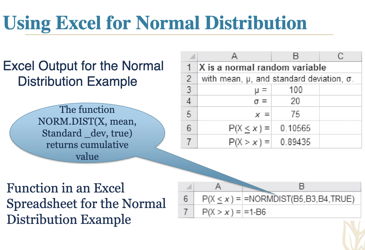
Excel on Normal distribution
Further examples utilizing the standard normal distribution properties.
Page 60
Haynes Construction Example:
Scenarios of construction completion times under normal distribution.
Page 61
Further exploration of construction probabilities and implications.
Page 62
Calculation of Z values to determine completion probabilities.
Page 63
Bonus calculations based on construction timelines and probabilities.
Page 64
Examination of completion probabilities in specific ranges.
Page 65
Standard Normal Table:
Probability values across standard deviations detailed.
Empirical Rule:
Distribution of values around the mean detailed in percentages.
For a normally distributed random variable with mean μ and standard deviation σ
Approximately 68% of values will be within ±1σ of the mean
Approximately 95% of values will be within ±2σ of
the meanAlmost all (99.7%) of values will be within ±3σ of the mean
F Distribution Overview:
Characteristics and applications of the F distribution explained.
The F Distribution (1 of 2)
It is a continuous probability distribution
The F statistic is the ratio of two sample variances
F distributions have two sets of degrees of freedom
Degrees of freedom are based on sample size and used to calculate the numerator and denominator
df1 = degrees of freedom for the numerator
df2 = degrees of freedom for the denominator
The probabilities of large values of F are very small
Consider the example:
– df1 = 5
– df2 = 6
– α = 0.05
• Check the F table
– Fα, df1, df2 = F0.05, 5, 6 = 4.39
• This means
– P(F > 4.39) = 0.05
The probability is only 0.05
F will exceed 4.39
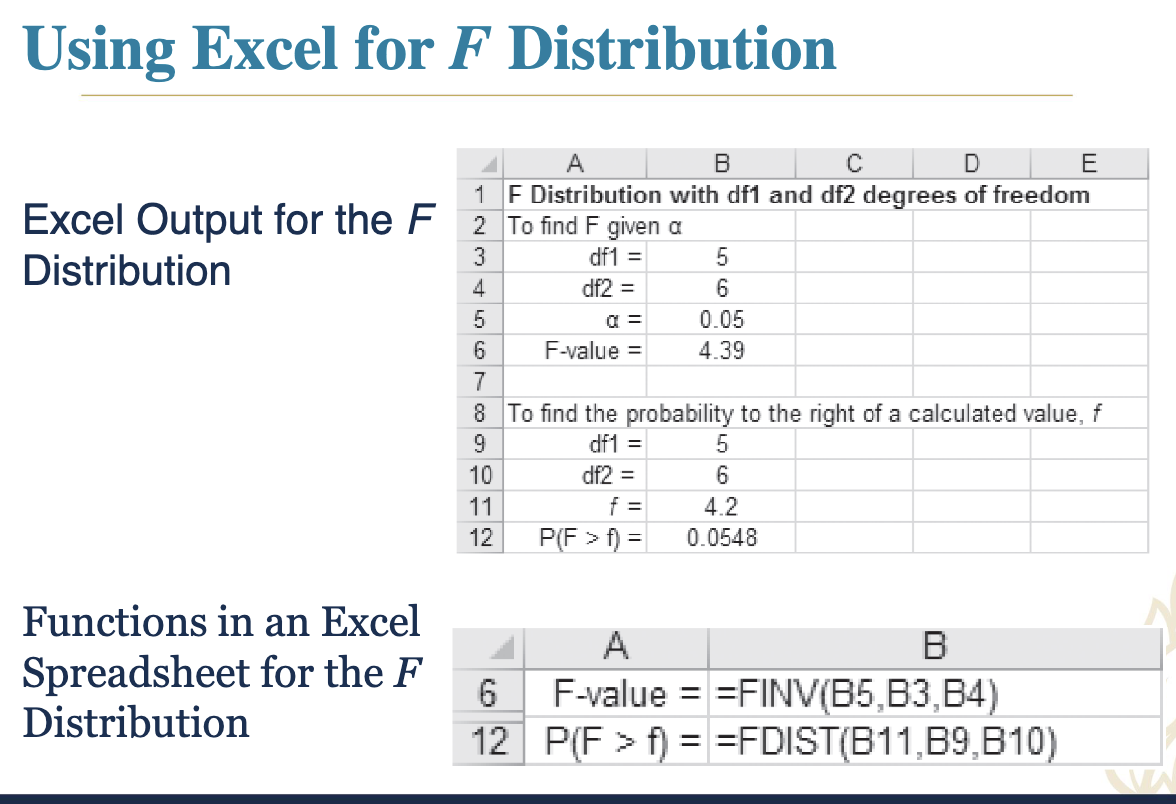
Using Excel for F distribution probability calculations discussed.
Exponential Distribution:
Defined and explained in relation to service times.
Also called the negative exponential distribution
A continuous distribution often used in queuing models
Probability function given by:
𝑓(X) = 𝜆𝑒−𝜆𝑥
where:
X = random variable (service times)
λ = average number of units the service facility
can handle in a specific period of time
(note: the textbook uses μ instead of λ)
e = 2.718 (the base of natural logarithms)Properties of the negative exponential distribution include:
Memoryless property: The future probability of an event is independent of the past.
The mean and variance are both equal to 1/λ, providing insight into expected service times and variability.
Extended properties of exponential distributions, including expected value and variance calculations.
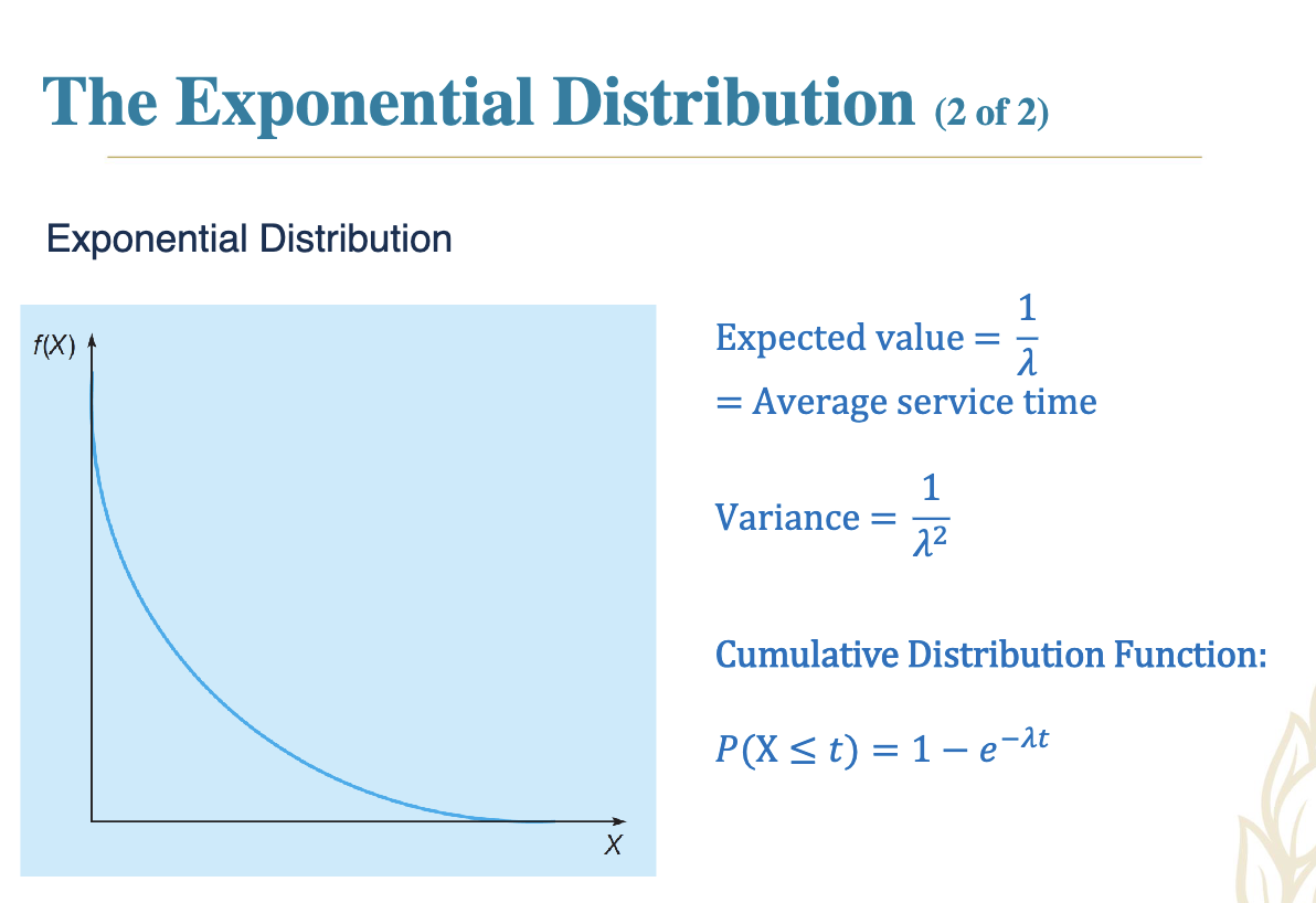
Expected value = 1/𝜆 = Average service time
Variance = 1/𝜆2Cumulative Distribution Function:
𝑃(X ≤ 𝑡) = 1 − 𝑒−𝜆𝑡This function describes the probability that a random variable X takes on a value less than or equal to t, illustrating the likelihood of service completion by time t.
Memoryless Property: The exponential distribution is unique in that it has no memory, meaning that the probability of an event occurring in the next time interval is independent of how much time has already elapsed.
This property is crucial in queueing theory, where it simplifies the analysis of systems. Understanding these concepts is essential for effectively modeling and predicting system behavior in various applications, including telecommunications and service industries.
Additionally, the exponential distribution is often used to model the time until the next event in a Poisson process, which is key in understanding the dynamics of random processes. In summary, mastering these probability concepts allows for better decision-making and optimization in processes that rely on random events.
Furthermore, the exponential distribution's probability density function is defined as f(t; \lambda) = \lambda e^{-\lambda t} for t \geq 0, where \lambda is the rate parameter, indicating the average number of events in a given time period. This function illustrates how the likelihood of an event occurring decreases exponentially over time, emphasizing the memoryless property that characterizes the exponential distribution.
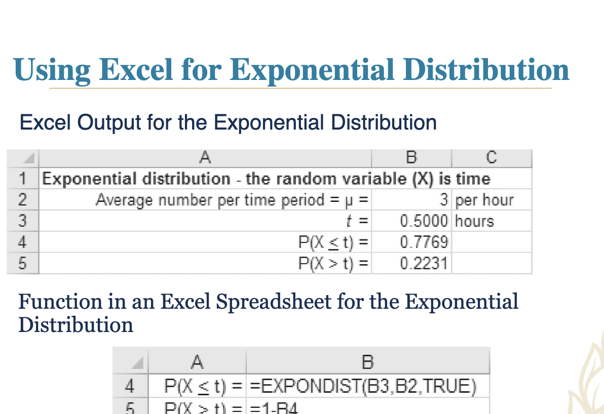
Arnold’s Muffler Shop Example:
Service time probabilities assessed through exponential distribution.
Installs new mufflers on automobiles and small trucks
– Can install 3 new mufflers per hour
– Service time is exponentially distributed
• What is the probability that the time to install a new muffler
would be ½ hour or less?
X = Exponentially distributed service time
λ = average number of units the served per time period =
3 per hour
t = ½ hour = 0.5 hour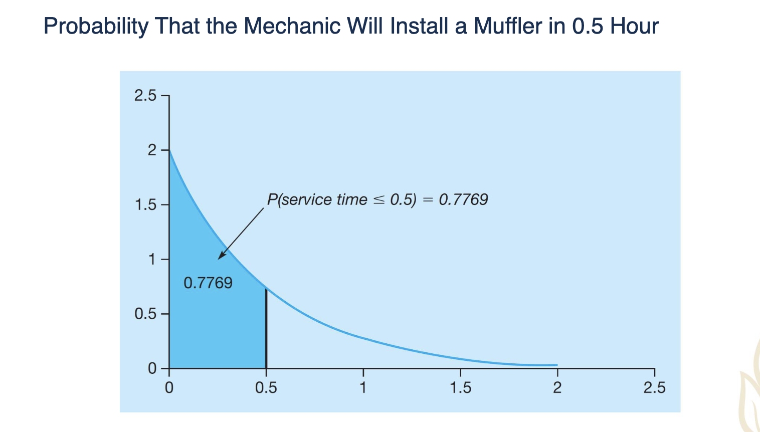
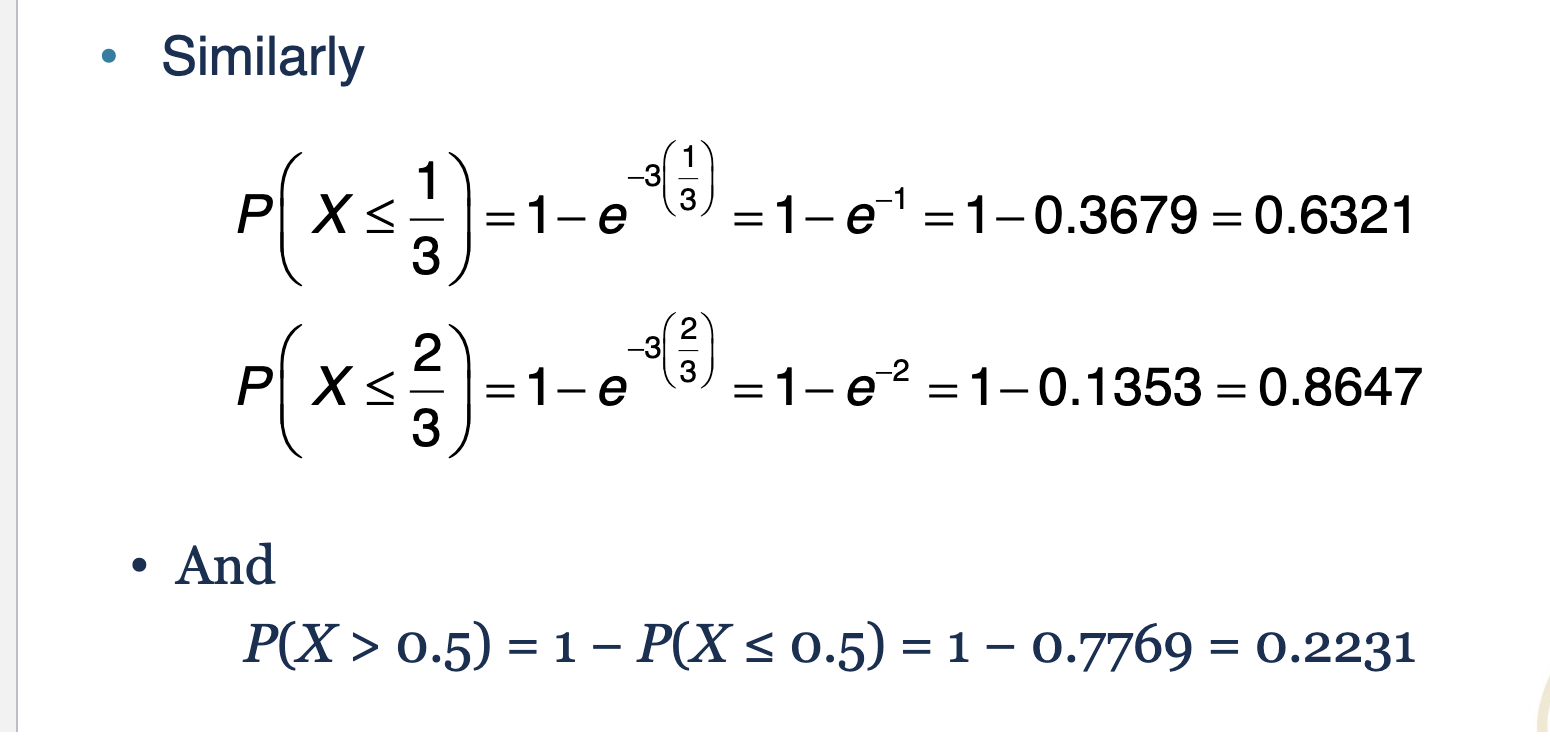
P(X ≤ 0.5) = 1 − e−3(0.5) = 1 − e −1.5 = 1 = 0.2231 = 0.7769
The expected value in this context represents the average service time, while the variance provides insight into the variability of service times across different customers.
Excel Exponential Distribution