Ecology
What is Ecology
Ecology relates back to natural history. Began with asking locals to describe animal behaviour they have noticed. 17-19th century saw the rise of natural historians, looking into evolution, biogeographical patterns, and taxonomy.
1866 - Ecology was coined as a term by Ernst Haekyl, with word origin relation back to the study of the home/environment.
Ecology: scientific study of interactions of organisms [with their environment and one another] that determine their distributions and abundances. Focus on interactions over species.
Ecological household: diverse, complex interactions among the living and nonliving parts of the planet that form it, is the focus. We want to uncover aspects of the house.
Ecosystem: a group of interacting organisms and their physical environment. Interactions occur between same organisms and different organisms.
Every animal has its own parasite or parasitic relationship, and food webs become infinitely more complex when you include parasites. When you change one trophic level or thing inside of an ecological population, there is a cascading effect, and other levels of interactions will be affected.
Ecology in the Anthropocene
Humans have changed earth so much that it is impossible to do pure ecology without looking into human implications and climate change. The world changing effects everything, every species, including us.
Diseases work the same way as predator and prey relationships, and medecine has made enormous progress.
One health: the combination of taking care of public health (medecine, hospitals, cures) and environmental health (global warming).
There are a few way to help environmental health by ecologists have been defined as being affected: climate change, overexploitation, land use change, invasive species, species mass extinctions, homogenization of habitats.
We have seen rise in: GDP, methane, population, energy use, carbon dioxide, nitrogen, surface temperature, ocean acidification, tropical forests being lost.
Ecology subdivisions
Biospheres
Individuals
Populations
Communities
Ecosystems
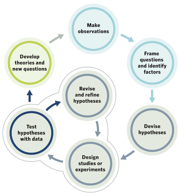
How we study ecology
Observation and Natural History
Foundation of ecology. Focus of observation and description of species. No hypotheses or typical scientific method. Scientific validity is expected by looking more into broad patterns on a different scale.
We still see this in other ways of studying ecology, its principles continuously pops up.
National Ecological Observatory Network (NEON): collections of data on abiotic factors in order to aid in standardized work.
Experimental Ecology and Null hypothesis Testing
Harder in ecology than lab sciences. Species interactions are not linear in ecology, they are instead evolving, which caused problems.
Avoiding “ad-hoc fallacies”: a story or narrative of observed patterns, described as “just-so”, “cuz it makes sense”.
We have seen certain species interaction have a ± relationship, which can cause “population cycling” - where the populations of each species will fluctuate in opposite rounds of each other.
Hypotheses aren’t great because of all the different effects on population cycling (resources, climate, species interactions)
Scientists cannot prove, they can only disprove.
Focal factors: key aspects of ecological experiment.
Multiple Hypothesis Testing and Best-Fit Comparisons
Experiments cannot be replicated due to many factors changing and evolving (no control): expensive, forest fires, ethically problematic, logistically problematic.
This is why we look at everything, and then try to conclude a best-fit comparison with a ton of potential hypotheses.
Advantages: can make use of large amounts of available information, allows for simultaneous experimentation, acknowledges uncertain, accommodate real world complexities.
We cannot look into sea lice in a fish farm, so we use our data to assume rates of sea lice in fish farms based on multiple hypotheses (does it increase, decrease, stay same).
We test “relative weight of supporting data”.
Ecological modelling
Does not require manipulation, allows to see what altering a factor would have on ecological dynamics.
Models are not reality - can be helpful in understanding.
May be conceptual or mathematical (which may be analytical or simulation based).
Conceptual model: Theoretical, various components in relationship with each other. Formalized idea of how things work. Look at energy, water, species, resources, logical connections, how resources pool and change by season. We analyze a set of question about a situation - this affects that and that affects this (rock, paper, scissors).
Mathematical model: What parts are most important to include in a model and what should be graphed. Change in population size is birth minus death.
Analytical model: using math equations and values to understand a change or phenomenon.
Simulation model: predict a model’s performance through running a computer program for a mathematical model to see all the different ways it could end up or last.
Organisms and their Environment
Biosphere: focus of ecologists; all living organisms on the earth, plus the environment in which they live.
Physical environment determines resources, and how a species can and may survive there. Species are best adapted to where they evolved. The weather patterns will help predict what lifeforms exist where. Tropic lines are similar to how global temperature map is set up.
Climate = long term, changes directionally in climate change over time.
Weather = current state of temperature, precipitation, etc.
Physical realizations determine energy rays.
Sun rays work based on how much of the rays energy is diffused
Hottest at equator because the sun is not diffused.
Earth’s axis is tilted, which increases
Northern hemisphere is leaning towards sun during the summer.
Sunlight is main source of energy on earth, explains shallow water in tropics having high biodiversity.
There are 5 physical principles to explain patterns
Equator gets the most total solar radiation
Hot air is lighter, so it rises.
Air pressure lowers as altitude increases.
Compression heats up air, expansion cools air down.
Warm air holds water, water vapour is visible in breath on cold days due to condensation in your hot breath.
Looking at the equator → rainforest
There is a lot of sun, hot air being pulled up, pressure lowers, air expands cooling down the air and releases water, causing it to rain.
With air on the top, it moves north and south, sinking about 30 degrees away. Deserts in the 30 degrees away. Then wet-dry pattern repeats every 30 degrees away (30, 60, 90).
North and south pole are 90 degrees away.
Predicting climate
We would expect all rainforest at one band, then all desert at the next, but there are various other effects with determine climate and biome.
Coriolis Effect
The earth rotates, giving object on earth a speed. North pole has low rotational speed, equator has high rotational speed.
Windspeeds are determined by this, and they determine ocean currents. Westerlies and tradewinds will cause currents to turn in a specific direction (depends on hemisphere and winds in region)
You may find high pressure areas, with warm water coming up.
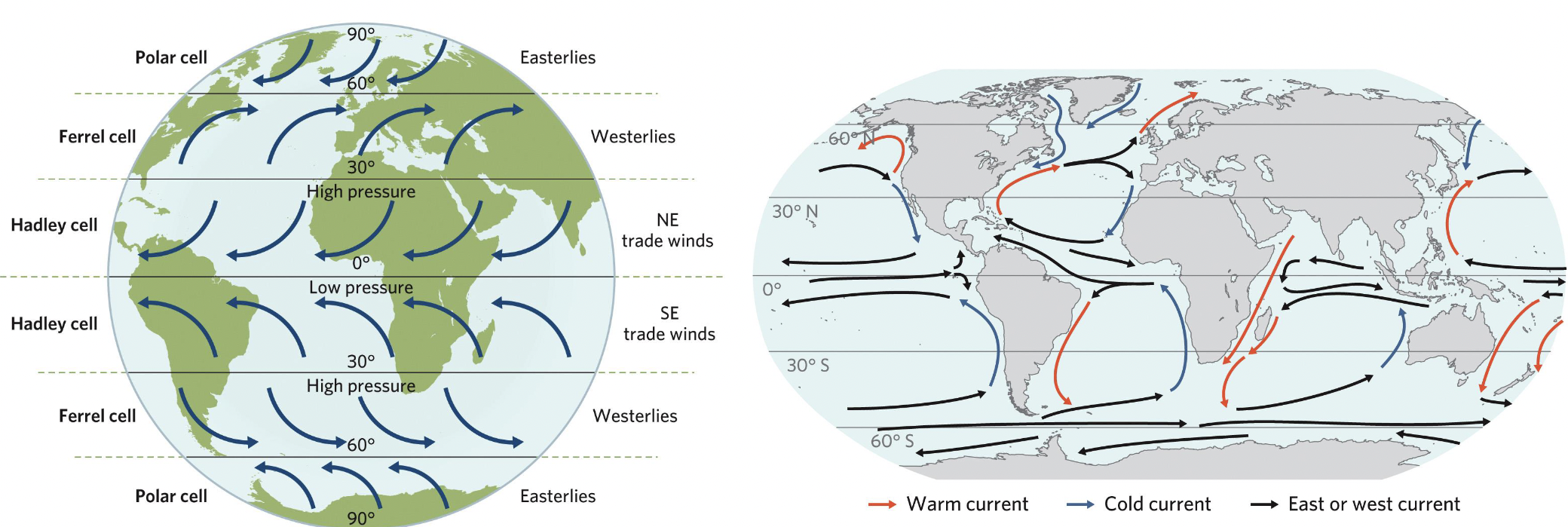
Hadley cells: Circles of cells moving air and is responsible for rainforests at equator
hadley-hadley: wet
hadley-ferrel: dry
Ferrel cells: Dry warm air that sank down and suck up moisture in desert.
ferrel-polar: wet
Polar cells: produce high pressure area at each polar region. Results cold, dry air returning to earth’s surface, why poles can be considered desert
Polar-polar: dry
Topography
Rain shadow. Wind coming into the ocean, forces the air up. Pressure will decrease and release everything on ocean side of mountain. Dry air moves past mountain, we call this the rain shadow.
Continental Effect
The heat capacity of soil is lower than the heat capacity of water (which is really high) (need lots of heat to heat up water). Areas surrounded by water do not change as much during the season, as the water works as a buffer for weather changing. Areas in the middle of continents have big swings and changes in seasons.
Transpiration
Plants have a cooling effect on other plants. Rainforests have large clouds of water, which creates their own weather. When plants heat up, they release water to cool down, and doing this a bunch generally cools the temperature down.
The different terrestrial biomes
Determined by the above, and the atmospheric cells in that region. Arctic has a lot of frozen water, but very little precipitation. Polar desert.
Species are best adapted to area in which they evolved. Tolerances of a species are determined by where they evolve. Niches will define their limiting variables. Red wood needs fog, so its around foggy areas.
Biomes are determined by → climate (temperature/water), soil (water availability, nutrient uptake), and plant communities (primary productivity, sunlight made to energy).
Most biodiversity is at the equator, and amphibian population rates can show biomes.
Climate diagrams: We often determine biome characteristics with a graph with two axis → temperature and precipitation. With proper scaling, we can see when there is enough water for plant growth and when evaporation outpaces precipitation.
Tropical Rainforest
Year round constant temperature, and lots of water year round. Precipitation outpaces.
Tropical dry forests
Year round constant temperature, with only one (long) season of water outpacing. Lots of biodiversity, but only during said season. Good soil for nutrient uptake in dry season.
Tropical savanna
Year round constant temperature, less water. Huge periods with no precipitation. Shorter season (1) with enough rain. Baked underlying soil.
Desert
30 degrees. Always limited water, can be hot or cold. Sparse plant life and animals. Polar cells.
Mediterranean scrubland
Cold currents buffer winter, areas kept pretty dry. Long period with no rain, short period with precipitation outpacing. Cool wet winters, hot dry summers.
Temperate grasslands
Temperature differs in winter and summer months, with always just enough or just not enough precipitation, they’re always towing the line.
Temperate forests
Temperature differs in winter and summer months, with always enough precipitation to house a forest. Precipitation outpaces a lot in cooler months.
Boreal forests
Temperature differs in winter and summer, with lots of excess precipitation to house a forest. Characteristically a lot of needle-leave trees and plants.
Tundra
Year round of just getting enough water, but trees cannot be supported. Very low temperatures.
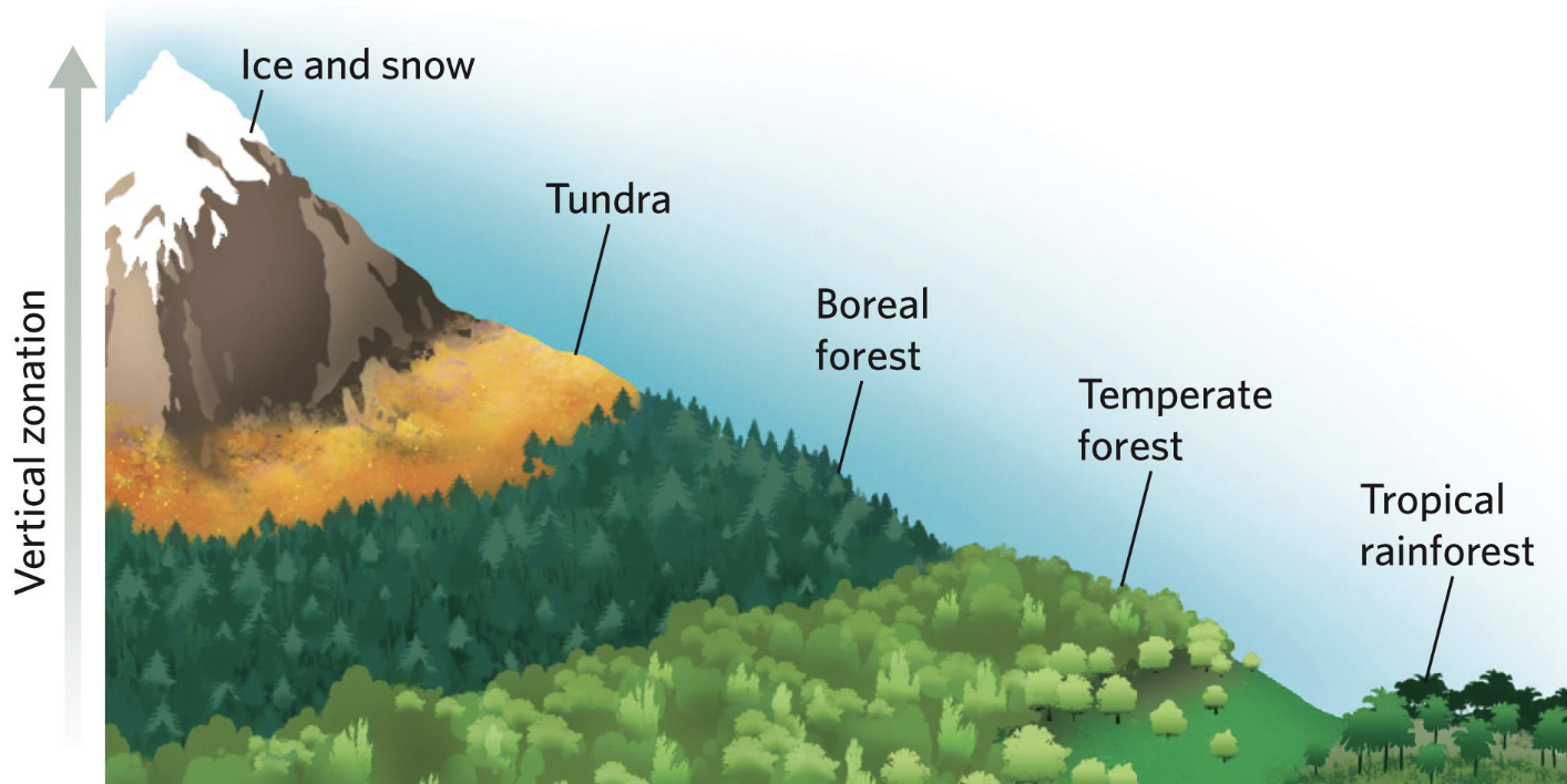
Biological zones on mountains
There are elevation gradients, where there are vegetation lands that mimic biomes.
 Aquatic biological zones
We determine aquatic biological zones using light, nutrient availability, temperature, structure of bottom surface, salinity, and physical movement.
Light determines photosynthesis
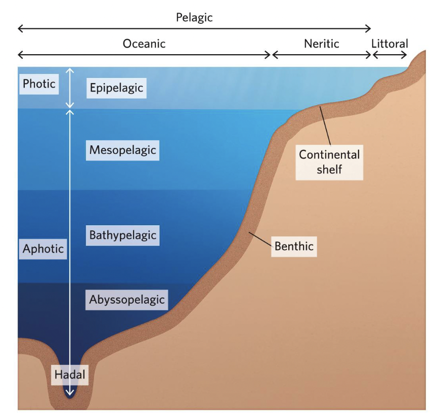
Marine zones
characterized by:
Light penetration determines photic zone (100-200m deep, depends on salinity)
Proximity to shoreline (littoral → neritic → oceanic)
Physical location (benthic on bottom, pelagic on ocean area)
Depth of pelagic zone
 Types of aquatic biological zones
Estuaries (juncture of rivers and oceans, fresh and saltwater mix), mangrove forests (trees in salinity, roots in water), seagrass beds (submerged flowering plants), coral reefs (creates structures, protists, lots of light, very fragile).
Coastal structure
Rocky substrate zone (kelp forests, underwater forest, fish rely on).
Sandy bottom zones (low biodiversity, nothing to hold onto).
We group oceanic zones as one zone because it is hard to understand, and a bunch of plankton luminate the oceans, showing its all connected, or that it’s at least similar.
Deep oceans have very little understood about them, with crush pressures as you move down to those depths.
Frozens seas make ice a habitat, on and underneath.
Freshwater zone - hard to classify, with river connecting to lake, to next river. Super limited zones. Forced directions for animals.
Human effects on global climate and biomes
Climate has changed a lot in time, with greenhouse gases having a large effect. This happens normally. We’re in the sixth mass extinction, like dinosaurs couldn’t handle shift in cold temperatures.
Greenhouse effect
Gases accumulate in the atmosphere, and reabsorption and radiation increases are causing increase in weather. We are adding too much greenhouse gas. It would occur naturally, these levels are unnatural. Bacteria can keep up, we cannot.
We have noted higher frequency of extreme weather events. Whole graph is shifting towards hotter. Sea levels are rising, and we expect 200 million climate refugees. Some stuff will die off, and some things will just take too long to come back, end up collapsing. This stuff shifts biomes. Non-deserts are desertifying, ending up with loss of grasslands.
Individuals: Physiology and Behaviour
Limiting factors and an organisms niche
Resources or conditions that limit growth, distribution and abundance of an organism or population within an ecosystem are known as limiting factors. This determines niche → a frog needs water, won’t be found in a desert.
Set of conditions and limiting factors determine if a species can be there. N-dimensional hypervolume (N for amount of limiting factors). This determines the ideal niche space for a species.
We are not doing equally as well in all spaces of a niche, and so we just optimize what we can and cannot. We have preferences, but with change we can persist more (types of food eaten, living in water and needing to swim around to find sources).
Ideas of stress, a species will not be doing best in all parts, and other species around may do well when they do poorly. This is called getting out-competed.
Principle of allocation - allocating resources to one function, limits allocation of resources to another function.
Energy is a limiting factor
We eat or parasitize energy, and have an energy budget. Energy budget differs by species.
No unlimited energy, so priorities are selected.
Intake = respiration + assimilation + reproduction + waste
Ingested = energy to get oxygen + growth structure or storage + sex + waste/heat
We take time to deploy strategies for eat, to determine efficiency.
P = E/C
Energy profitability = energy gained / energy cost associated with acquiring for
P indicates profitability, and should be above 1, the “breakeven point”. C is the search and handling cost.
Biomass - unused energy converted into tissues or growth stored as fat. Waste in terms of feces.
Polar bears need ice to hunt seals, without ice, there is longer fasting periods, more starvation, more bony, fewer and lighter cubs, increased cub mortality. When there is enough energy, you can assimilate and store energy for periods of no food, however with shorter periods of time to assimilate, and being force to live off less for more time, you only focus energy on reservation instead of reproduction/sex.
Semelparous - reproduce one in their lifetime
Iteroparous - organisms that produce many times (not always top priority)
Temperature is a limiting factor
There are different groups of species which determines preferred climates, and where is liveable.
Cold blooded
Poikilotherms: Don’t regulate at all, don’t care. Plants, marine fish.
Ectotherms: Using external factors to regulate. Amphibians, reptiles.
Warm blooded
Endotherms: Use behavioural thermoregulation + internal temperature
Homeotherms: able to maintain in a very narrow range
Non-homeotherms: not as good at maintaining in a range with crazy temperature.
Thermal performance curves are specific to one axis per niche space. They show where a species is at optimal temperature (for their metabolic rate, maintaining homeostasis), as well as where they begin to stop functioning, and where their lethal limits are. Lizards have a very specific pattern of moving in order to thermoregulate and keep within a safe range.
We see an increased spread of viruses and diseases due to climate change, where under hot conditions, mosquitoes develop a disease and these disease are moving up. A lungworm can parasitize a slug and will in turn parasitize muskoxen (they eat slugs), and will migrate up north, bringing the disease with them.
Climate envelope: focus on species physiology and where it currently is (compare all temperatures and what climate is like). Ignores mechanisms and how species got there.
Record where species is found
Determine climate of places, where species occurs
Look at climate map to see where these conditions occur/will occur in future
Thermal performance based of population models - estimate where a species could potentially occur with thermal constraints. R0 is important and defined as average offspring produced by an individual per lifetime. We look for where R0 <1 on the map.
Determine R0
Estimate thermal performance curves for each term in equation
Combine climate map projections with how R0 varies in different temperatures. We’re interested where R=1, as a way of seperating increasing and decreasing populations.
R0 may tell us where you can establish, but they may not establish there. They still need to walk there or they can walk away and stuff.
Even under good thermal constraints, species may not be able to get there, only as an invasive species potentially.
Resource utilization curves - n-dimensional hypervolume puts everything in equal play. We break up niche into multiple curves, what species do, not physiological requirements.
Population: Population Growth
Population - group of individuals living and interacting with one another in a particular area.
Abundances - number of individuals
Densities - abundance relative to the area occupied
Exponential graph - you can use these ecological graphs for cells spreads.
Obtaining population data
What do you count?
Individuals, characteristics, sex, stage of life.
Where do you count?
Must define population bounds. Natural geographic areas (island), or you may run into issues with highly mobile species leaving and rejoining bounds. Hotly debated how many polar bears can be highlighted so we look at genetics of discreet populations, long periods of time. Determine closed or open populations
How do you count?
We are limited to taking subsamples and extrapolating to how much we can estimate.
Ntotal/Atotal = Nsample/Asample
We extrapolate population of one area, to a larger total area and population
Ways to count
Counting signs of species (discreet species)
Reports by community like trappers and hunters, however can be biased because they focus on the biggest animals in a bunch
Sampling plots - going to coral reef and counting individuals in a plot
Line transect by sight or sound - more individuals you encounter, more likely there are. Encountering X amount in X amount of space.
Mark-recapture method - collect, mark, recapture, count
Can be done with camera traps, recognizing ocelot patterns in their coat as their ‘marks’
Can learn more information in video than just location, but also behaviour, health, eyes, migration, abundance, densities, habitat uses (weather, routine, solitude), birth and death rates, interspecies interactions.
Marked/Total = Recaptured/Captured
Bigger sample, bigger accuracy
Population Dynamics
Population growth
Beavers are an invasive species, and as an ecosystem engineer, they changed the environment and messed with a lot of species. It is too difficult to tell how many there will be in 50 years.
Discrete-time (geometric) population growth
Population abundance at t + 1, so really just one year in the future
Nt+1 = Nt + Bt - Dt + It - Et
We usually just regard our population as closed, and so we ignore immigration and emigration. Birth and death can vary by environment and population size changing. Where are the new beavers going to build dams? More individuals has an effect (carrying capacity). We assume birth and death are constant.
per capita death rate (d): death expected per year
per capita birth rate (b): births expected per year
Nt+1 = Nt(1 + b + d)
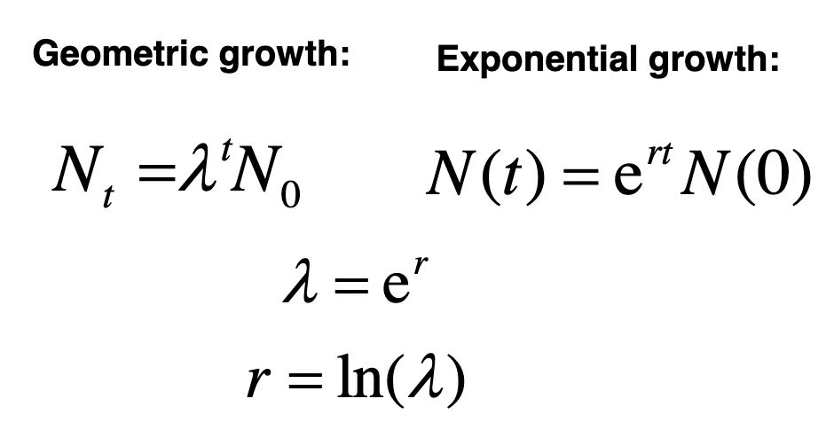
Nt+1 = Nt λ
λ = ( Nt+1 / Nt )1/t
Geometric Growth equation
Nt = N0 λt
Nt+2 = Ntλ2
λ < 1 population declines, λ = 1 population stays same, λ > 1 population increases
Same applies for r, but in terms of r>=<0)
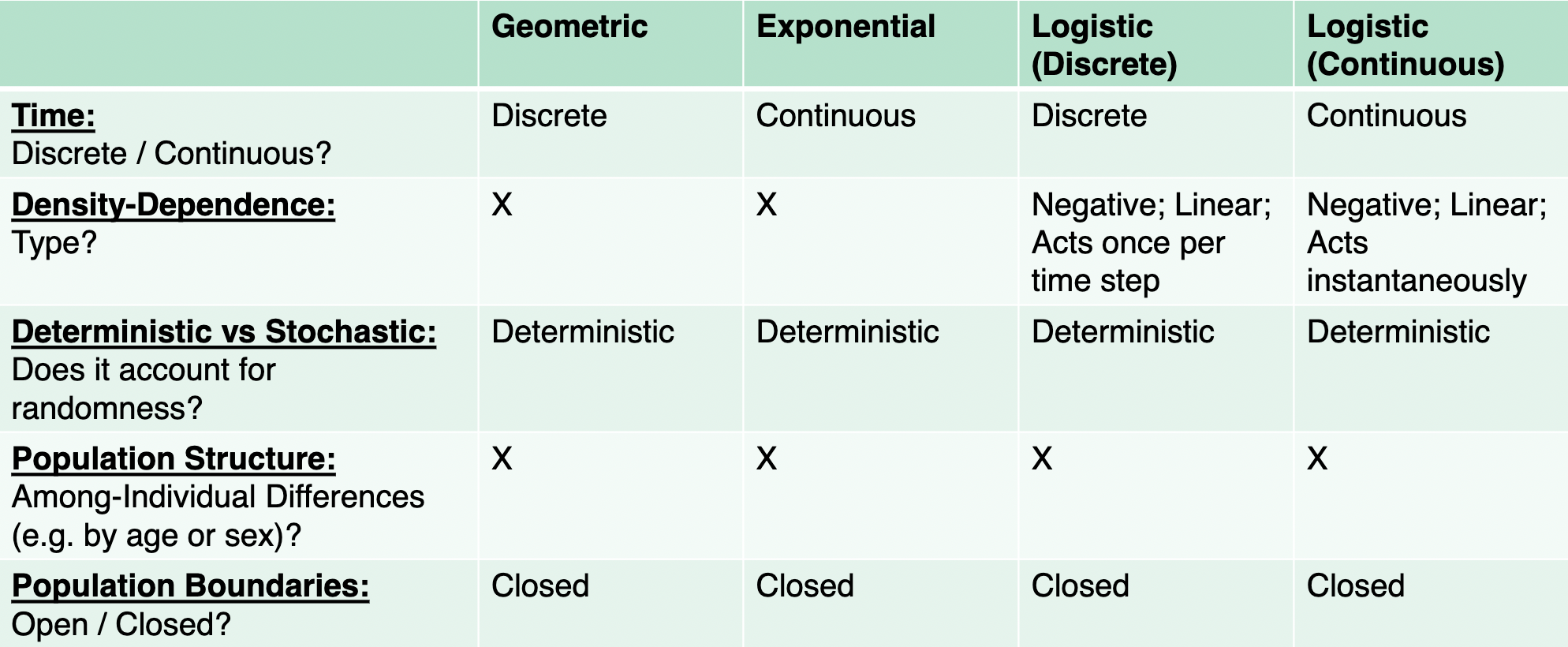
We assume (with geometric model of population growth) - closed population, discrete time period, no environmental effects, individuals are treated equal
Continuous-time model (exponential population growth)
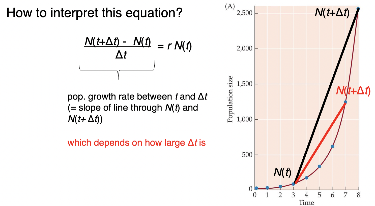
Accounts for population changes instantaneously. Most appropriate for species where population abundance changes continuously. It is not intuitive at once, but the idea is that instead of calculating population size from one to next, we question where we start from and rate of changing population.
Change per year = (Nt+1 - Nt) / 1 year = Nt (b-d) = (ΔN / Δt)
limt →0 (ΔN/Δt) = dN/dt, where d is derivative
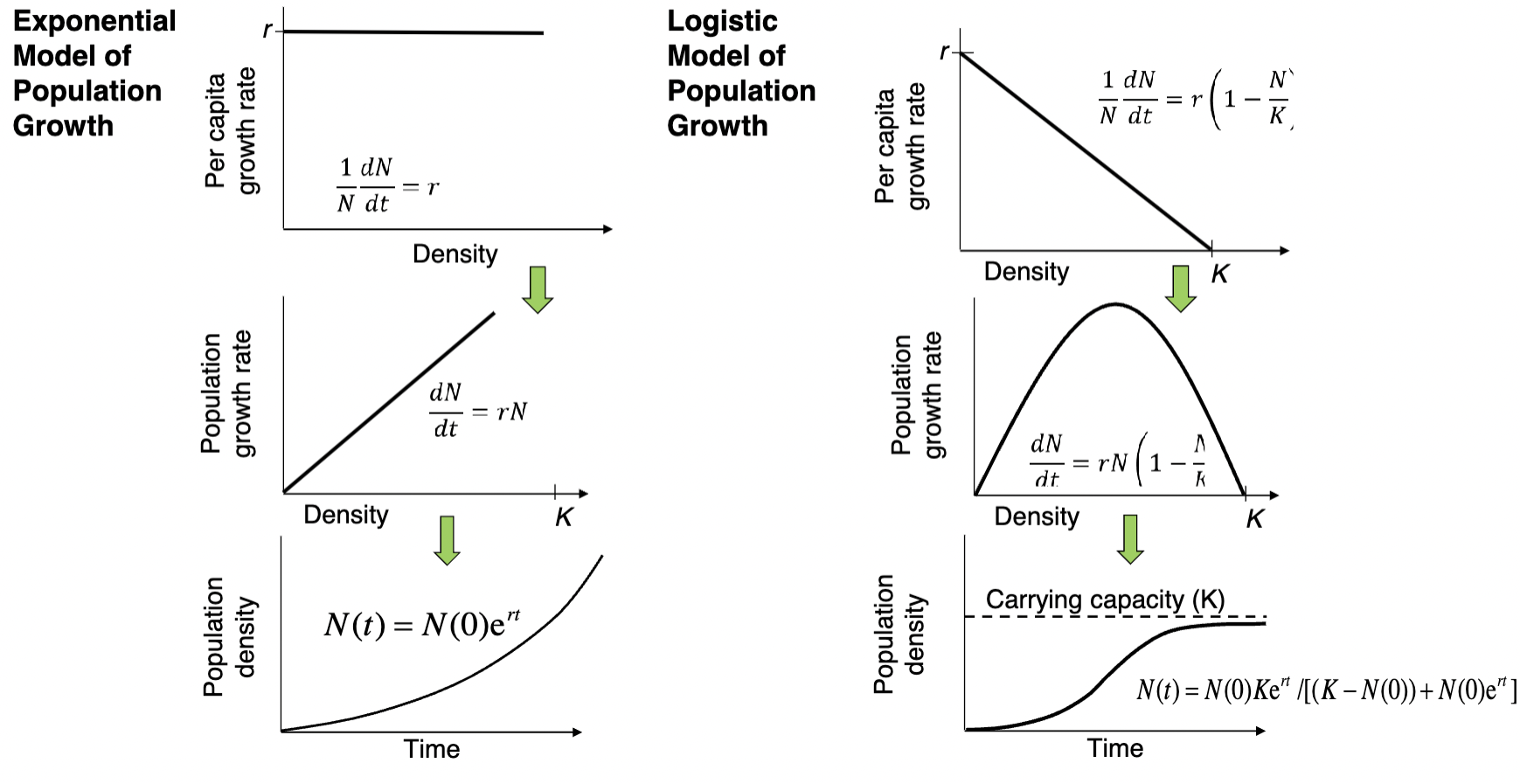
= rN, where r is the instantaneous per capita rate of population growth
 It is imperative that we check units when doing any of these equations.
Population regulation
Density-independent factors: Wildfires, natural climate events. Will happen independently of how many individuals there are in a population.
Density-dependent factors: Limited resources, survival rates decline, emigration will occur. Logic works regardless of if birth rates or linear or not.
Continuous time, with carrying capacity
Nt = (N0 Kert) / [(K - N0) + N0ert)]
 Logistic growth (assumes per capita population growth rate declines as N increase)
dN / dt = rN(1 - N/K), where K is the carry capacity.
Here we get the S curve bringing us to carrying capacity.
Assumption of logistic model: closed population, changes occur continuously, independent of environment, individuals are treated equal, growth rate is linear with population density, density-dependent acts instantaneously.
Discrete-time, density-dependent population growth
rdisc = b - d = λ - 1
Nt+1 = Nt + Nt rdisc [(K - Nt)/K]
Different types of graphs
S-shaped population - low intrinsic population growth rate (rdisc > 0)
Damped oscillation - follows normal s-curve, then spikes and tampers off. (rdisc < 1)
Stable limit cycle - population is up and down rapidly (rdisc << 1)
Chaos - s, then damped, then stable, then damped, weird (rdisc <<< 1)
Butterfly effect; small difference on initial conditions drastically changes results of population trajectory
Population: Spatial Dynamics
Population Dynamics at Low Densities
Very low density can be positive, because you’re doing good and not approaching issues that come with carrying capacity. However, going too low can lead to extinction which is a big prevalent issue.
How do extinctions actually happen
Ones that particularly bother small population, positive-density dependence is not a realistic measure of of how a population goes extinct.
Allee effect - population density increases at small population sizes. per capita growth rate increases as population density increases at a small population sizes.
Effect logistic model of population growth, by spiking increase until point and then tailoring off.
While low densities are positive, it makes it hard to find mates, losing cooperative predator defense (school of fish), environmental conditioning (marmots cuddling for warmth).
Smaller populations are vulnerable to inbreeding (no options) and genetic drift) - issue means mixing harmful recessive alleles, or bringing bad alleles elsewhere, losing good alleles and keeping bad ones.
Stochastic events (stochasticity) - random events that fluctuate population sizes. Cause fluctuations in population size around deterministic trends. Increase risk of extinction; larger fluctuations and smaller populations.
Environmental: changes average growth rate from one time to next because of random changes in environmental conditions.
Demographic: averages don’t change much, however individuals don’t follow averages, leading to fluctuations.
Extinction vortex - all of the above issues, leads to loss genetic diversity, reduction in individual fitness and population adaptability, and then higher mortality and lower reproduction, and finally leading to extinction.
helping may just make it worse. You can’t just reintroduce birds, it has to be a good amount of birds.
Age/Stage-Structured population dynamics
We shouldn’t be treating all individuals the same. Can work, but often doesn’t.
Humans → kids aren’t having kids as much, composition of population may vary and that will change birth rates.
Survivorship curves
Type I - many live young and die old (humans)
Type II - super average age structure, individuals dying at a consistent rate (seagull)
Type III - many die young, and those that live live for a good amount of time.
We must calculate the fecundity and survival rates of the three stage classes (pre-reproductive, reproductive, post-reproductive). Stage makes more sense than age, cuz they vary in length.
px - probability to survive and go to next stage
gx - probability to survive and stay in class
px + gx = sx , survival rates
fx - fecundity rate
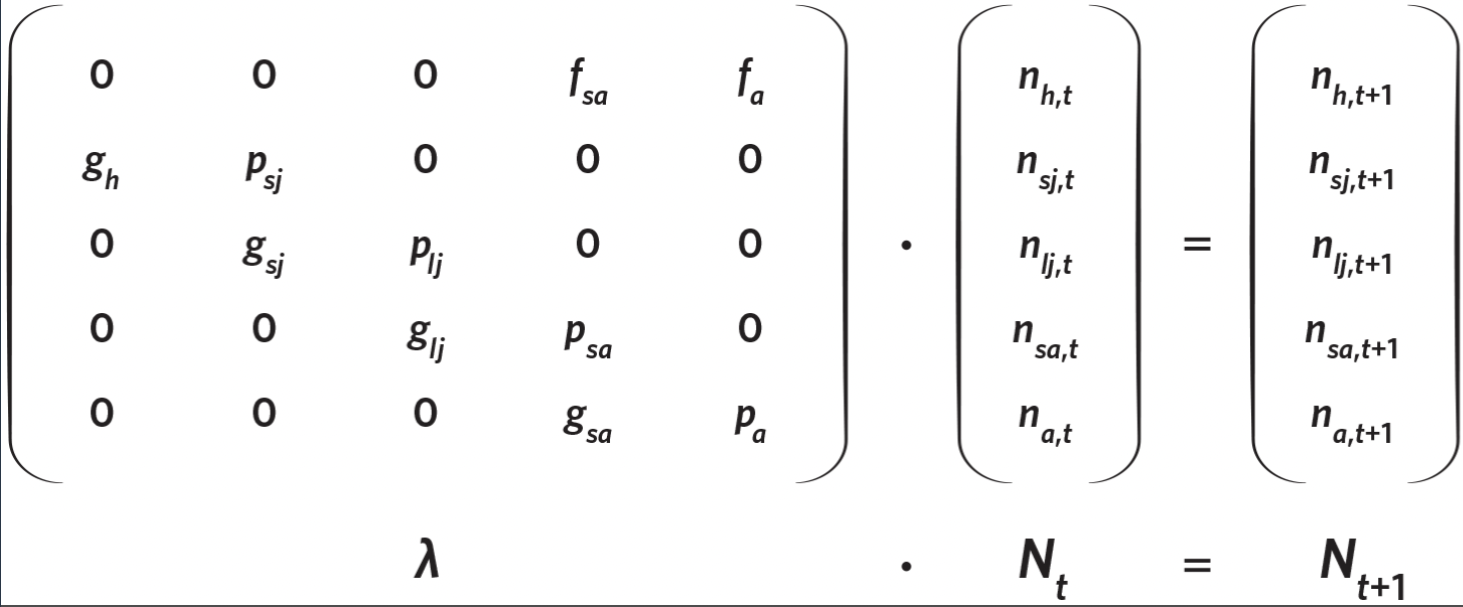
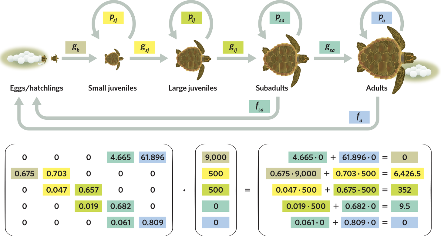 Lambda * current population vector. Multiply them in that order. Stable stage distribution: proportions of individuals in each age class remain constant over time. Dictated by survival and fecundity parameters. Population growth continues based on lambda.
Proportions don’t change after awhile. Increasing small juveniles-adults increases turtle survival rate. We can analyze where to target which will have the biggest effect. Keeping grown turtles alive has greatest effect.
Spatially structured population dynamics
Movement can occur for many reasons and it affects population dynamics
Dispersal: Movement by an individual to an unknown or unidentified location, without returning
Increase fitness
Natal dispersal, breeding dispersal.
Migration: Movement of many individuals at approx same time, predictable, time of year or life stage, round trip events or round trip over generations.
One location may provide better survival success, and the other better reproductive success
Outcome of migration must outweigh the costs.
The above can both shift species ranges
Metapopulation - doesn’t take death and growth rate into account.
Lights blinking on and off. Subpopulations bet colonized and then go extinct. Spatial structures can allow for good movement.
Subpopulations linked by dispersal.
p=0, all patches are empty; p=1, all patches are occupied.
Levins metapopulation model
rate of colonization → cp(1-p)
c amount that reach patch, p proportion of patches that send colonists.
dp/dt = cp(1-p) - ep
total rate of change in the proportion of occupied patches, p, is therefore given by the differential equation.
c>e, metapopulation persists, c<e metapopulation goes extinct.
e → value for extinction
Metapopulations need to be managed as a whole, can persist with extinct subpopulations assuming habitat patches permit dispersal and recolonization, losing patches implies number of occupied patches will also decrease in metapopulation.
Decreasing connectivity can aid in curbing disease, while increasing can aid in conservation of endangered species.