Chapter 12 (Cozby), + Chapter 4, Chapter 6, Chapter 8 (Davis & Smith)

There are four types of validity: Construct validity, internal validity, external validity, and conclusion validity. Statistical conclusion validity was defined as the accuracy of the statistical conclusions drawn from results that are based on statistical analyses.

There are two branches of statistics: descriptive statistics and inferential statistics. Descriptive statistics are procedures used to summarize a set of data. Inferential statistics are procedures used to analyze data after an experiment is completed. It is used to determine if the independent variable has a significant effect.

There are two ways in which statistics help us understand data collected in research investigations:

1. statistics are used to describe the data,

2. statistics are used to make inferences and draw conclusions about a population on the basis of a sample data.

Scales of measurement

Whenever a variable is studied, the researcher must create an operational definition of the variable and devise two or more levels of the variable. The levels of the variable can be described using one of four scales of measurement: nominal, ordinal, interval, and ratio.

The levels of nominal scale variables have no numerical, quantitative properties. The levels are simply different categories or groups.

9Variables with ordinal scale levels exhibit minimal quantitative distinctions. We can rank order the levels of the variable being studied from lowest to highest. With an ordinal scale, the intervals between items probably are not equal.

With an interval scale variable, the intervals between the levels are equal in size. There is no absolute zero point that indicates an “absence” of the variable.

Ratio scale variables have both equal intervals and an absolute zero point that indicates an absence of the variable being measured.

An important implication of interval and ratio scales is that data can be summarized using the mean, or arithmetic average.

Describing results

There are three basic ways of describing the results:

1. Comparing group percentages: this is useful when a key variable is being measured on a nominal scale. After describing data, the next step would be to perform a statistical analysis to determine whether there is a statistically significant difference between the two groups, or if the differences in the sample are due to chance.

2. Correlation scores of individuals on two variables: this is needed when you have an interval or ratio scale of measurement. In this circumstance, the individuals are measured on two variables, and each variable has a range of numerical values.

3. Comparing group means: Much research is designed to compare the mean responses of participants in two or more groups.

   For all types of data, it is important to understand your results by carefully describing the data collected. We begin by constructing frequency distributions.

Frequency distributions

A frequency distribution shows how often each score occurred. Along with the number of individuals associated with each response of score, it is useful to examine the percentage associated with this number.

By examining frequency distributions, you directly observe how your participants responded. You can see what scores are most frequent, and you can look at the shape of the distribution of scores. You can tell whether there are any outliers - scores that are unusual, unexpected, or very different from the scores of other participants.

By grouping frequencies and creating a grouped frequency distribution, you can reduce the number of categories and the meaning of your data becomes clearer.

Graphing frequency distributions

Pie charts divide a whole circle into “slices” that represent relative percentages. Pie charts are particularly useful when representing nominal scale information. Pie charts are most commonly used to depict simple descriptions of categories for a single variable.

Bar graphs use a separate and distinct bar for each piece of information.

Frequency polygons use a line to represent the distribution of frequencies of scores.

A histogram uses bars to display a frequency distribution for a quantitative variable. In this case, the scale values are continuous and show increasing amounts on a variable.

Histograms, bar graphs, and frequency polygons graphically depict distributions - ways in which the frequencies are spread out or distributed in the various categories. Statisticians use several different terms to describe the different shapes these distributions can assume.

When a distribution has one prominent category or high point, researchers call it a unimodal distribution. A bimodal distribution has two prominent high categories or high points, whereas a multimodal distribution has several prominent categories or high points.

A symmetrical, unimodal, bell-shaped distribution that has half of the scores above the mean and half of the scores below the mean (and is asymptotic), is known as a normal distribution.

When the scores in your distribution tend to cluster in one of the tails (i.e., a cluster of high scores or a cluster of low scores), the distribution is skewed. A skewed distribution is a non symmetrical distribution. Such distributions have one tail that is more spread out and long; this is the tail that has the fewer scores on it.

When there is a cluster of lower scores, the smaller, more spread-out tail will be on the right (i.e., fewer high scores); this configuration is called a positively skewed distribution.

When there is a cluster of high scores, the smaller, more spread out tail will be on the left side (i.e., fewer small scores); this configuration is called a negatively skewed distribution.

Descriptive statistics

Descriptive statistics allow researchers to make precise statements about the data. We use descriptive statistics when we want to summarize a set or distribution of numbers in order to communicate their essential characteristics.

Two statistics are needed to describe the data:

A single number can be used to describe the central tendency, or how participants scored overall. Another number describes the variability, or how widely the distribution of scores is spread.

Central tendency

A central tendency statistic tells us what the sample, as a whole, or on the average, is like.

There are three measures of central tendency:

1. The mean of a set of scores is obtained by adding all the scores and dividing by the number of scores. The mean is an appropriate indicator of central tendency only when scores are measured on an interval or ratio scale, because the actual values of the numbers are used in calculating the statistic.

2. The median is the score that divides the group into equal halves. The median is appropriate when scores are on an ordinal scale, because it takes into account only the rank order of the scores.

3. The mode is the most frequent score. The mode is the only measure of central tendency that is appropriate if a nominal scale is used.

The median or mode can be a better indicator of central tendency than the mean if a few unusual scores bias the mean. The median may be a better choice as your measure of central tendency when your distribution of scores is skewed.

When we calculate the mean, we take the value of each number into account. Although the medians for two distributions may be the same, the mean may not be. Because the mean takes the value of each score into account, it usually provides a more accurate picture of the typical score and the is the measure of central tendency favored by psychologists.

Variability

Variability is the extent to which scores spread out around the mean.

One measure of variability is the range, which is simply the difference between the highest score and the lowest score.

Another measure of variability is the standard deviation, which indicates the average deviation of scores from the mean. The standard deviation is the square root of the variance. The standard deviation of a set of scores is small when most people have similar scores close to the mean. The standard deviation becomes larger as more people have scores that lie farther from the mean value.

In order to obtain the standard deviation, we must first calculate the variance, S². You can think of the variance as the single number that represents the total amount of variation in a distribution. The larger the number, the greater the total spread of the scores.

A deviation score is the difference between a score (X) and the mean (M), showcased by the following formula:

X-M

We can now define variance as the average of the sum of the squared deviation scores.

(X-M)²

Because we need to sum the squared deviation scores, we have to add  Σ to the formula

 Σ(X-M)²

We then divide the sum of the squared deviations by the number of scores (N). This gives us the deviation score formula for variance:

This can be tedious, and most researchers therefore prefer to use the raw score formula to calculate the variance:

1. Square each raw score, then sum the squared scores

2. Sum the raw scores, then square this sum. Divide the squared sum by N.

3. Subtract the product obtained in Step 2 from the total obtained in Step 1.

4. Divide the product obtained in Step 3 by N.

To calculate the standard deviation, all the have to do is take the square root of the variance.

As with the variance, the larger the standard deviation, the greater the variability or spread of scores.

Interpreting the standard deviation

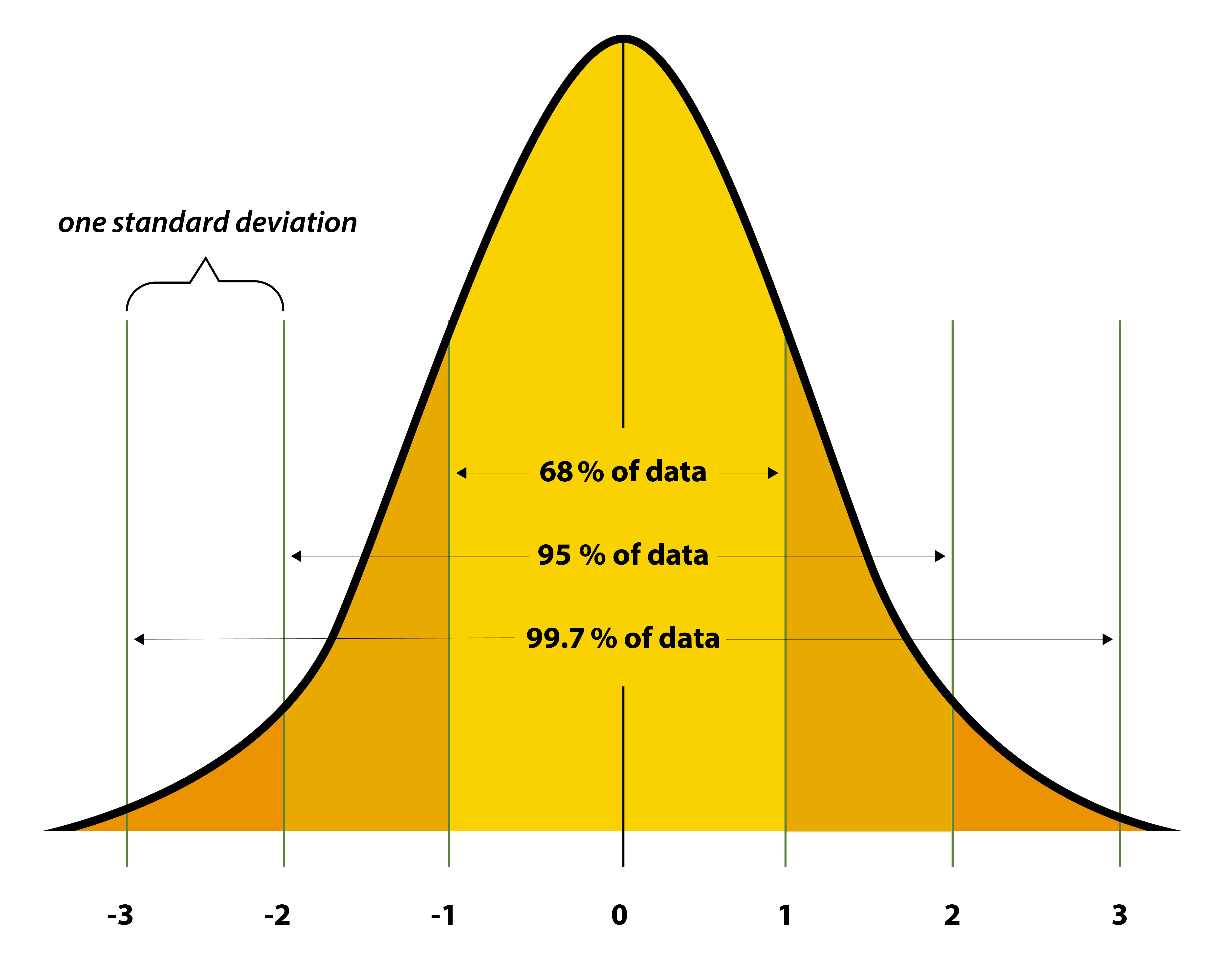
In the normal curve, the majority of scores tend to cluster around the measure of central tendency, wth fewer and fewer scores occurring as we move away from it. Normal distributions and standard deviations are related. Distances from the mean of a normal distribution can be measured in standard deviation units.

34.13% of all the scores in all normal distributions occur between the mean and one standard deviation above the mean and one standard deviation below the mean (added together, this makes it so that approximately 68.28, or 68%, of the data lies within 1 SD of the mean). Another 13.59% occur between one and two standard deviations above the mean, and one and two standard deviations below the mean (adding up to 95.44% of all the scores occurring between two SDs from the mean). And then exactly 2.28% of the scores occur beyond two standard deviations above and below the mean.

As we move away from the mean (either above or below), the scores become progressively different from the mean. When a normal distribution is taller and peaked, the standard deviation will be smaller because the scores are definitely clustered around the mean.

Graphing relationships

A common way to graph relationships between variables is to use bar graphs or line graphs. The levels of the independent variable are represented on the horizontal x-axis, and the dependent variable values are shown on the vertical y-axis.

Correlation coefficients: describing the strength of the relationships

A correlation coefficient is a statistic that describes how strongly variables are related to one another. The Pearson product-moment correlation coefficient is used when both variables have interval or ratio scale properties. Values of a Pearson r can range from 0.00 to 1.00. A correlation of 0.00 indicates that there is no relationship between the variables.

Pearson r Correlation Coefficient

The Pearson r provides two types of information about the relationship between the variables. The first is the strength of the relationship; the second is the direction of the relationship.

Mathematically, we can define r as the average of cross-products of z-scores. Stated as a formula:

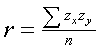
Using this formula to calculate r means that you would have to convert all scores on both the X and Y variables to z scores. Then, you would multiply the two scores for each pair of scores and sum these products. Finally, you would divide this total by the number of paired scores (N).

Scatterplots

In a scatterplot, each pair of scores is plotted as a single point in a diagram. The values of the first variable are depicted on the x-axis, and the values of the second variable are shown on the y-axis.

Important considerations

There are two important factors to consider when thinking about correlation.

1. Restriction of range: If the range of possible values is restricted, the magnitude of the correlation coefficient is reduced. The problem of restriction of range occurs when the individuals in your sample are very similar on the variable you’re studying.

2. The two variables could have a nonlinear relationship: If the relationship is curvilinear, the correlation coefficient will not indicate the existence of a relationship.

Effect size

Effect size refers to the strength of association between variables. It refers to the size or magnitude of the effect an IV produced in an experiment or the size of the magnitude of the correlation.

Generally speaking, as our sample size gets larger, the critical value needed to achieve significance becomes smaller. There is an inverse relation for the degrees of freedom (as they are based on sample size). As df become larger, all the table values become smaller.

The Pearson correlation coefficient is one indicator of effect size: the strength of the linear association between two variables.

It is sometimes preferable to report the squared value of a correlation coefficient. Instead of r, you will see r². Researchers refer to the squared correlation coefficient, r², as the coefficient of determination. This reason is that the transformation changes the obtained r to a percentage. The percentage value represents the percentage of variance in one variable that is accounted for by the second variable. The r² value is sometimes referred to as the percent of shared variance between the two variables.

r² x 100 = percentage of the variance accounted for by the correlation

Regression equations

Regression equations are calculations used to predict a person’s score on one variable when that person’s score on another variable is already known. Generally speaking, regression refers to the prediction of one variable from our knowledge of another variable. We label the variable that is being predicted as the Y variable, and refer to it as the criterion variable. We label the variable that we are predicting from as the X variable and refer to it as the predictor variable. In other words, we use X to predict Y. The general form of a regression equation is:

Y = a+bX

where Y is the score we wish to predict, X is the known score, a is a constant, and b is a weighing adjustment factor that is multiplied by X.

The regression equation can be used to produce a graph showing the straight line describing the linear relationship.

When researchers are interested in predicting some future behavior (called the criterion variable) on the basis of a person’s score on some other variable (called the predictor variable), it is first necessary to demonstrate that there is a reasonably high correlation between the criterion variable and the predictor variable.

The regression line is a graphical display of the relation between values on the predictor variable and predicted values on the criterion value.

Multiple correlation and regression

A technique called multiple regression is used to analyze the relationship between a criterion variable and more than one predictor variable.

A multiple correlation (symbolized as R instead of r) is the correlation between a combined set of two or more predictor variables and a single criterion variable.

A multiple regression equation can be calculated that takes the following form:

Y = a+b1X1 + b2X2+…bNXN

Mediating and moderating variables

Mediation

The word mediation means that something is coming between two forces. In research, a mediating variable is hypothesized to be intervening between variable X and variable Y.

In a mediation model, the independent or predictor viable affects a mediating variable. The mediating variable then affects the dependent or criterion variable.

Moderation

Moderation implies restraint or change. In research, a moderating variable changes or limits the relationship between variable X and variable Y. Specifically, the relationship depends on the level of the moderator variable M.

Third variables

Researchers face the third-variable problem in non experimental research when some uncontrolled third variable may be responsible for the relationship between two variables of interest. The third variable is responsible for an apparent relationship between variable X and variable Y, and X and Y are, in fact not related at all when the effect of the third variable is taken into account.

Multiple regression can be used to statistically control for the effects of third variables.

Interpreting correlation coefficients

When they are referring to research results, statistically significant means that a research result occurred rarely by chance. In other words, some other factor, such as the IV in an experiment, was effective and likely produced the results under consideration.

A standard for statistical significance at the .05 level means that researchers consider that a statistical results is significant when it occurs by chance 5 times out of 100.