knowt logo

Week12-ECMT1020_Ch6-8-1

Introduction to Model Misspecification

  • Classical assumptions for least squares (LS) include:

    • Regressor: xi is nonstochastic, regressor is fixed, not random.

    • Model Specification: Correctly specified as yi = β1 + β2xi + ui.

    • Error Term: ui has mean zero, E[ui] = 0.

    • Variance Condition:

    • Homoskedasticity: E[u²i] = σ²; error term is independent across observations, proving efficiency.

    • The error term is independent across i, and thus E[uiuj] = 0 if i not equal to j.

    • Normal Distribution: ui follows a normal distribution.

Model Misspecification and Omitted Variable Bias

  • Model misspecification relates to the failure to include relevant variables or the inclusion of irrelevant ones.

Omitted Variable Bias

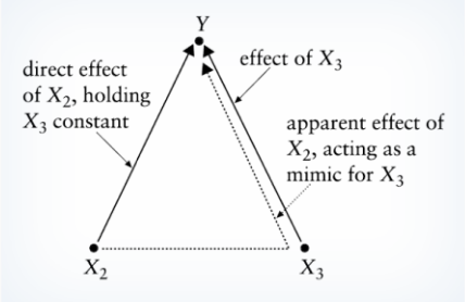
  • Scenario: True model: yi = β1 + β2xi + β3wi + ui, but regressor wi is omitted leading to:

    • Estimated model: yi = β1 + β2xi + ei, where ei = β3wi + ui.

    • OLS estimator of β2 (denoted by β2-hat) is biased and its expectation is:

      Figure 1

      *Swap e with w and expand it, we will have also an OLS estimate included the third coefficient

      Estimator of B2 with marginal effect of the interaction term B3

Recall that an estimator is unbiased if its expectation is equal to its population counterpart:

  • Conditions for unbiasedness:

    • β3 = 0 (wi has no effect).

    • cov(xi, wi) = 0 (no correlation).

      —> These two conditions forces the B2 estimator above to be unbiased.

We can view the estimator of variable w as the slope coefficient that have marginal effect of x and w on dependent variable.

Bias Direction

  • Omitted Variable Bias:

    this is the omitted variable bias

  • Direction of the omitted variable bias depends on the signs of B3 and fitted-cov(xi, wi)

    • Positive bias if both β3 and cov(xi, wi) are positive.

    • Negative bias if β3 is negative while cov(xi, wi) is positive.

    • R² in mispecified models will be lower than in correct model.

  • Alternative estimations like instrumental variable (IV) estimation are suggested.

Inclusion of Irrelevant Regressors (Ch 6.3)

  • When irrelevant regressors are included in a model that have insignificant effect to the dependent variable, the omitted variable bias arises.

    • True model: yi = β1 + β2xi + ui, included zi in your regression and obtain the following OLS:

      Figure 2

Note that:

Then sub into the figure 2:

expand the covariance to see the u with mean 0

  • If ui has mean zero, OLS remains unbiased as long as xi and zi are non-stochastic.

Irrelevant regressor doesn’t change much of the original regressor. It caused the regression model to be a little inefficient, T-statistic decreases while variance increases, p-value increases.

Proxy Variables (Ch 6.4)

  • Definition: A proxy variable is used in regression analysis to stand in for another variable that’s difficult to measure or unavailable, having properties similar to those of missing variable.

  • Example: Can’t measure intelligence directly, might use education as proxy.

  • True model with proxy:

    • Original: yi = β1 + β2xi + β3wi + ui;

    • Use proxy, imagine can’t observe wi directly:

      yi = β1 + β3α1 + β2xi + β3α2w∗i + ui. (subbed in)

  • Result: Parameters of interest is β3α2 rather than β3, R² remains unchanged.

  • It is impossible to solely identify B3 without further information a2.

  • t-stats for w* identical to w.

The new proxied regression will not affect estimation results of the coefficient of xi.

Stochastic Regressors

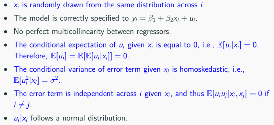
With the stochastic regressors, meaning it will no longer fixed and will be random, we have the following assumptions:

  • what’s different here is that we have stochastic regressor, no multicollinearity between regressors, conditions for expected value, variance, distribution and independence.

Efficiency and Properties of OLS Estimators

Under these new conditions, particularly under conditional expected value and no perfect multicollinearity —> OLS estimator is unbiased.

To see this, consider simple linear regression:

OLS estimator B2 satisfies that:

looking at Figure 1, there are no B3 in this linear regression

Because ai is a function of xi, E[a|x] = ai, we have:

Similarly:

  • Given conditional homoskedasticity condition, the OLS estimator has the smallest variance among all the unbiased estimator, thus BLUE.

  • As sample increases, OLS estimators converge to true parameters without needing normality of error terms.

  • As sample size increases, we don’t need normality condition of u|x to conduct statistical inference on OLS estmator, this is because of asymptotic normality of the OLS estimator.

Measurement Errors (Ch 8.4)

Measurement errors occurs when variables used in the models aren’t measured accurately, arise very often due to systematic error.

Suppose:

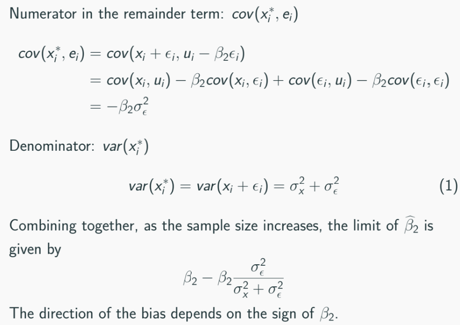
Now you don’t have the true regressor xi, and you have xi*, contaminated observation of xi such that:

The variable e is measurement error with mean zero and variance of σ2e. e is assumed to be independent of xi and ui, that is:

Since we cannot observe xi*. we use:

Thus the OLS will be:

As sample size increases B2^ will converge to:

Measurement error in dependent variable

Measurement error in the dependent variable does not generate a bias of the OLS estimator.

Suppose:

With measurement error in dependent variable, of mean zero and variance σ2e:

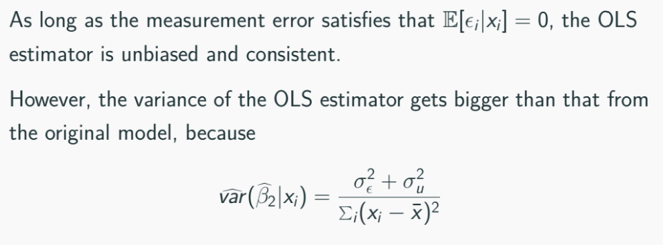
The OLS estimator will reduces to:

Measurement errors in dependent variables does not affect consistency of OLS estimator.

Measurement Error & Omitted Variable Bias

  • Measurement errors, when combined with omitted variables, result in inconsistent OLS estimates.

  • IV estimation recommended; utilizes external, correlated variables to ensure accurate parameter estimation.

V

Week12-ECMT1020_Ch6-8-1

Introduction to Model Misspecification

  • Classical assumptions for least squares (LS) include:

    • Regressor: xi is nonstochastic, regressor is fixed, not random.

    • Model Specification: Correctly specified as yi = β1 + β2xi + ui.

    • Error Term: ui has mean zero, E[ui] = 0.

    • Variance Condition:

    • Homoskedasticity: E[u²i] = σ²; error term is independent across observations, proving efficiency.

    • The error term is independent across i, and thus E[uiuj] = 0 if i not equal to j.

    • Normal Distribution: ui follows a normal distribution.

Model Misspecification and Omitted Variable Bias

  • Model misspecification relates to the failure to include relevant variables or the inclusion of irrelevant ones.

Omitted Variable Bias

  • Scenario: True model: yi = β1 + β2xi + β3wi + ui, but regressor wi is omitted leading to:

    • Estimated model: yi = β1 + β2xi + ei, where ei = β3wi + ui.

    • OLS estimator of β2 (denoted by β2-hat) is biased and its expectation is:

      Figure 1

      *Swap e with w and expand it, we will have also an OLS estimate included the third coefficient

      Estimator of B2 with marginal effect of the interaction term B3

Recall that an estimator is unbiased if its expectation is equal to its population counterpart:
  • Conditions for unbiasedness:

    • β3 = 0 (wi has no effect).

    • cov(xi, wi) = 0 (no correlation).

      —> These two conditions forces the B2 estimator above to be unbiased.

We can view the estimator of variable w as the slope coefficient that have marginal effect of x and w on dependent variable.

Bias Direction

  • Omitted Variable Bias:

    this is the omitted variable bias

  • Direction of the omitted variable bias depends on the signs of B3 and fitted-cov(xi, wi)

    • Positive bias if both β3 and cov(xi, wi) are positive.

    • Negative bias if β3 is negative while cov(xi, wi) is positive.

    • R² in mispecified models will be lower than in correct model.

  • Alternative estimations like instrumental variable (IV) estimation are suggested.

Inclusion of Irrelevant Regressors (Ch 6.3)

  • When irrelevant regressors are included in a model that have insignificant effect to the dependent variable, the omitted variable bias arises.

    • True model: yi = β1 + β2xi + ui, included zi in your regression and obtain the following OLS:

      Figure 2

Note that:

Then sub into the figure 2:

expand the covariance to see the u with mean 0

  • If ui has mean zero, OLS remains unbiased as long as xi and zi are non-stochastic.

Irrelevant regressor doesn’t change much of the original regressor. It caused the regression model to be a little inefficient, T-statistic decreases while variance increases, p-value increases.

Proxy Variables (Ch 6.4)

  • Definition: A proxy variable is used in regression analysis to stand in for another variable that’s difficult to measure or unavailable, having properties similar to those of missing variable.

  • Example: Can’t measure intelligence directly, might use education as proxy.

  • True model with proxy:

    • Original: yi = β1 + β2xi + β3wi + ui;

    • Use proxy, imagine can’t observe wi directly:

      yi = β1 + β3α1 + β2xi + β3α2w∗i + ui. (subbed in)

  • Result: Parameters of interest is β3α2 rather than β3, R² remains unchanged.

  • It is impossible to solely identify B3 without further information a2.

  • t-stats for w* identical to w.

The new proxied regression will not affect estimation results of the coefficient of xi.

Stochastic Regressors

With the stochastic regressors, meaning it will no longer fixed and will be random, we have the following assumptions:
  • what’s different here is that we have stochastic regressor, no multicollinearity between regressors, conditions for expected value, variance, distribution and independence.

Efficiency and Properties of OLS Estimators

Under these new conditions, particularly under conditional expected value and no perfect multicollinearity —> OLS estimator is unbiased.

To see this, consider simple linear regression:

OLS estimator B2 satisfies that:

looking at Figure 1, there are no B3 in this linear regression

Because ai is a function of xi, E[a|x] = ai, we have:

Similarly:

  • Given conditional homoskedasticity condition, the OLS estimator has the smallest variance among all the unbiased estimator, thus BLUE.

  • As sample increases, OLS estimators converge to true parameters without needing normality of error terms.

  • As sample size increases, we don’t need normality condition of u|x to conduct statistical inference on OLS estmator, this is because of asymptotic normality of the OLS estimator.

Measurement Errors (Ch 8.4)

Measurement errors occurs when variables used in the models aren’t measured accurately, arise very often due to systematic error.

Suppose:

Now you don’t have the true regressor xi, and you have xi*, contaminated observation of xi such that:

The variable e is measurement error with mean zero and variance of σ2e. e is assumed to be independent of xi and ui, that is:

Since we cannot observe xi*. we use:

Thus the OLS will be:

As sample size increases B2^ will converge to:

Measurement error in dependent variable

Measurement error in the dependent variable does not generate a bias of the OLS estimator.

Suppose:

With measurement error in dependent variable, of mean zero and variance σ2e:

The OLS estimator will reduces to:

Measurement errors in dependent variables does not affect consistency of OLS estimator.

Measurement Error & Omitted Variable Bias

  • Measurement errors, when combined with omitted variables, result in inconsistent OLS estimates.

  • IV estimation recommended; utilizes external, correlated variables to ensure accurate parameter estimation.

robot