1.1.3 - Demand, Supply, and Market Equilibrium

Demand Definition - Syllabus 1.1.3(a)

• \
• ==Demand===Amount of a good consumers are willing & able to buy, at a specific price & specific point in time.^^Market demand^^

• \

• \

• \

• 

• \

• \

• \

  

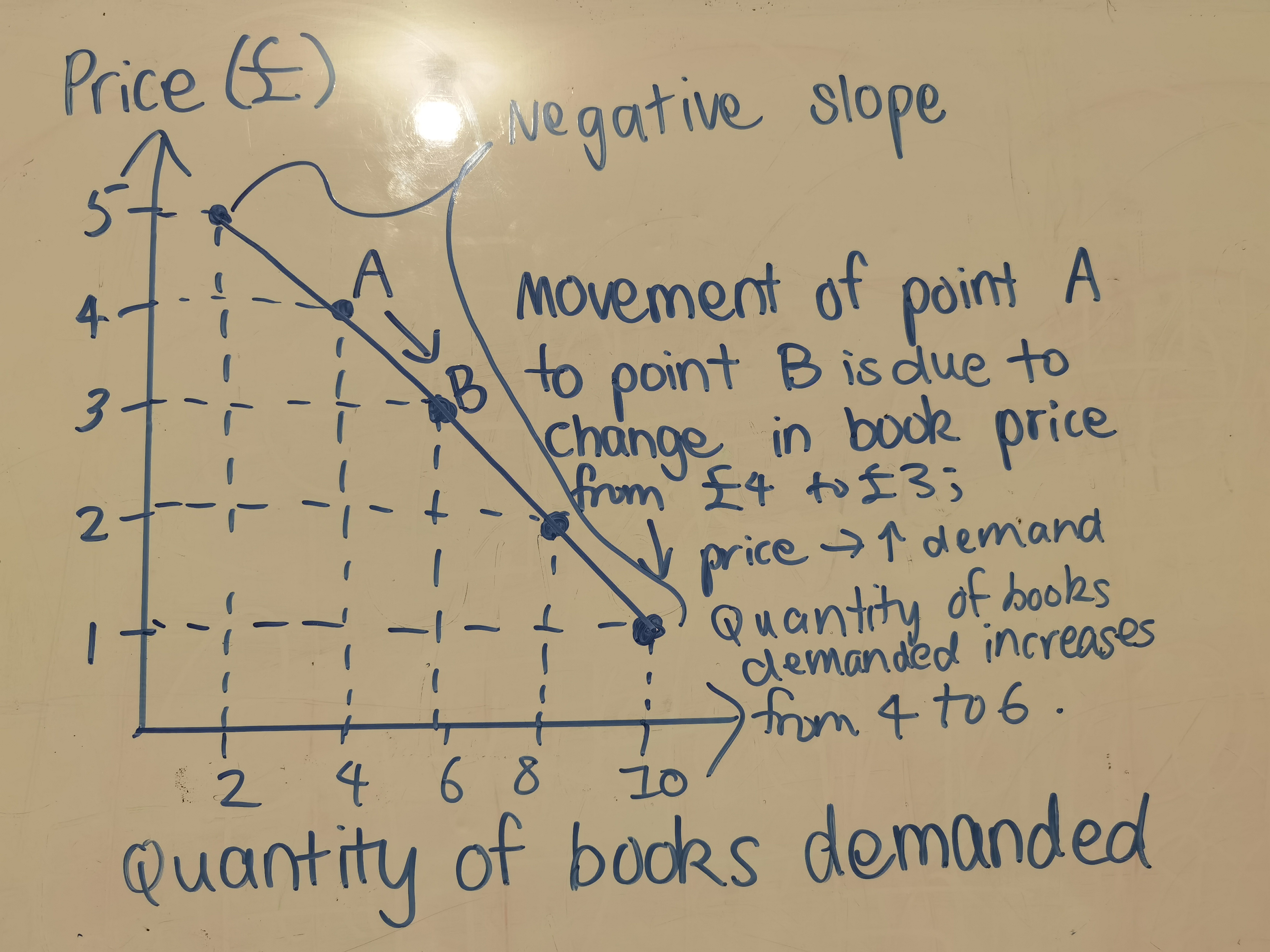
• = The sum of all individual demand schedules in the market.Demand Curve - Syllabus 1.1.3(b)==Demand curve == = Graph showing amount of a good consumers are willing & able to buy at different prices.==Negative slope == → Goes down from left to right →

• \

1. \

2. \

3. \

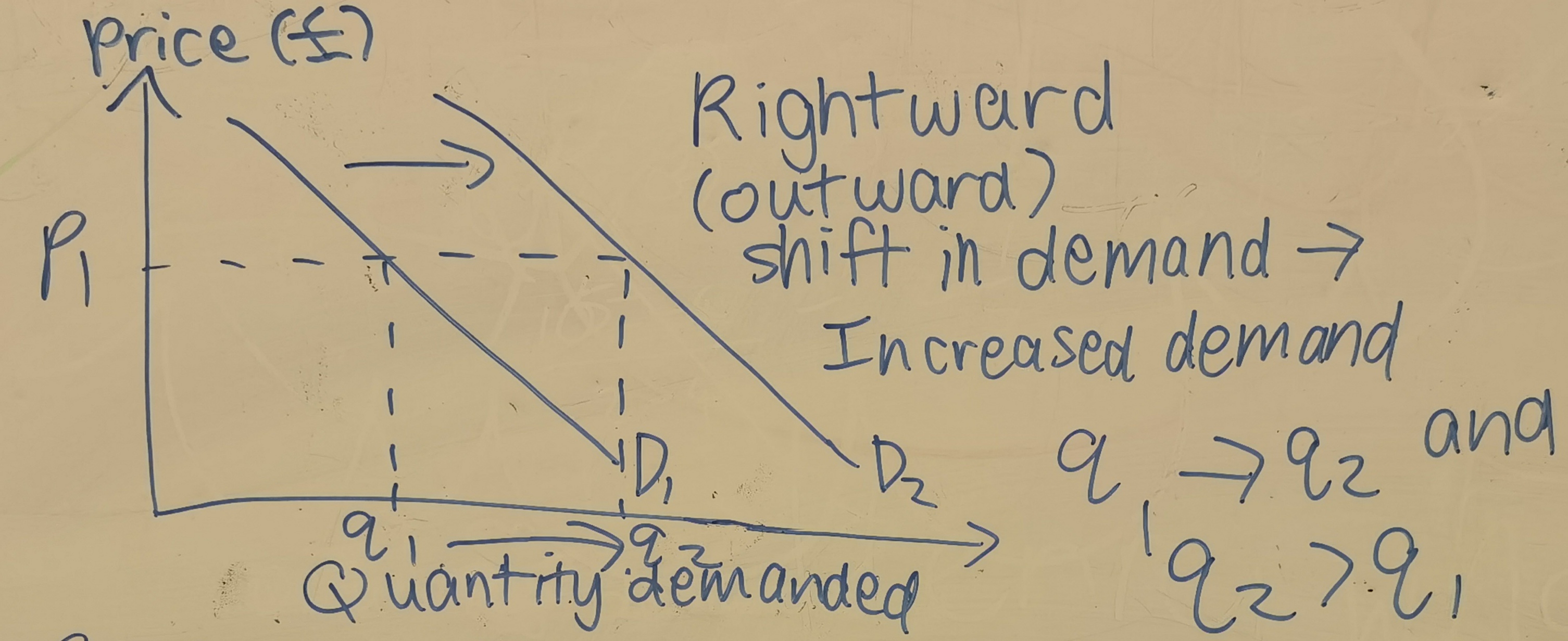
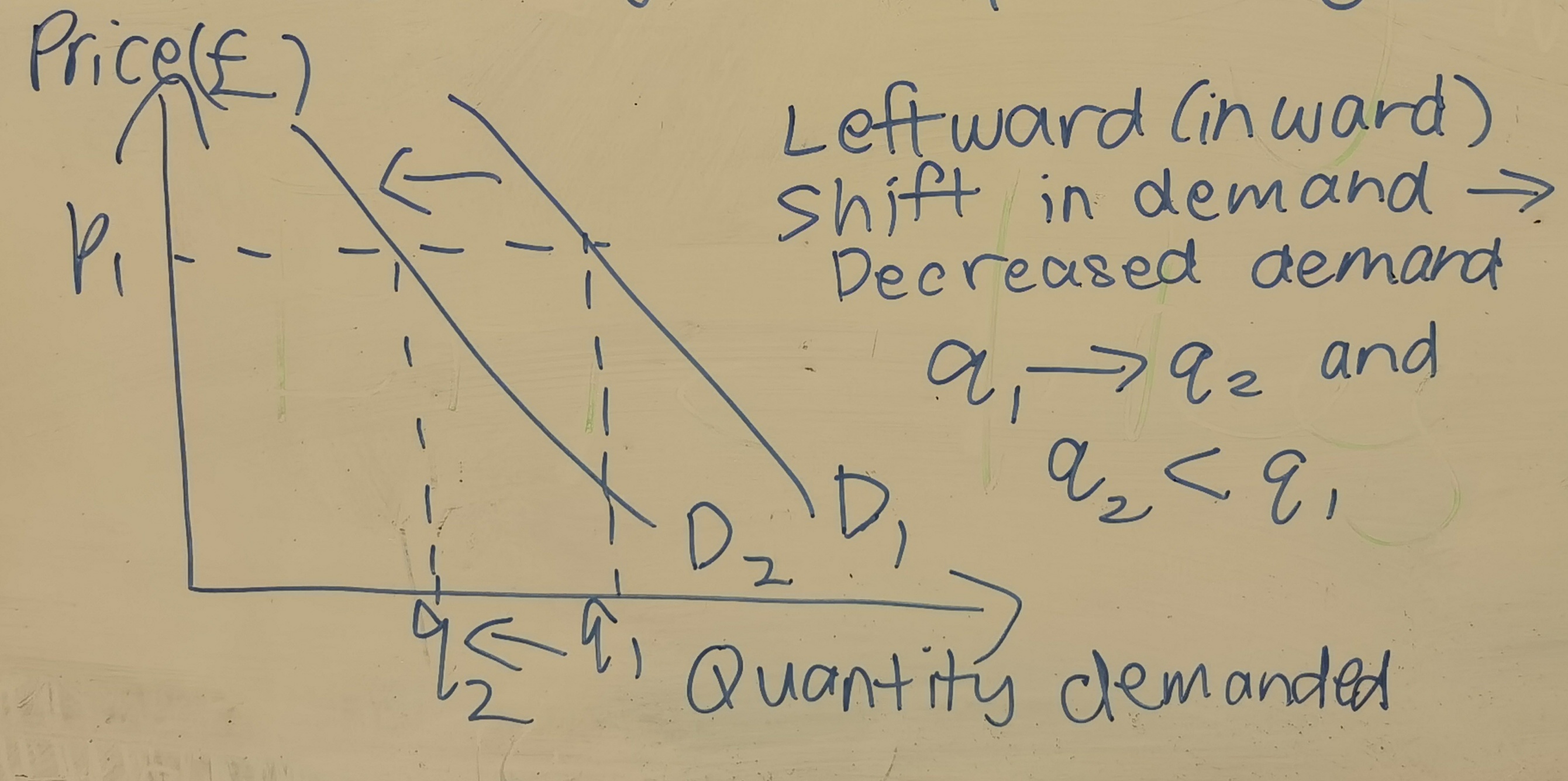
4. ==**Inverse relationship**** == for price & amount demanded:↑ price → ↓ quantity demanded↓ price → ↑ quantity demanded^^**Change in price of originally-investigated good**^^→ Movement along demand curve==**Factors NOT related to change in price of originally-investigated good*** == → Shift in demand curve==**Rightward/outward demand shift*** * == → ↑ demand==**Leftward/inward demand shift*** == → ↓ demandPrice is ALWAYS on==**y-axis.**==Quantity demanded is ALWAYS on==x-axis.==Example:==Demand schedule

   1. \

   2. *== = Table of the quantity demanded of a good at different price levels, used to calculate expected quantity demanded and plot points on demand curve.Example:Price (£) of BooksQuantity of books demanded11028364452Factors causing Shifts in the Demand Curve - Syllabus 1.1.3(c)Use==FISCAD== acronym:==Fashion & Tastes==Consumer trends & tastes affects the popularity, and therefore demand, of certain goods/services.E.g. Scrunchy trend → ↑ Demand for scrunchies==

      1. \
      2. \

   3. \

   4. \

   5. \

   6. \

5. \

6. \

7. \

8. \

9. \

10. IncomeDisposable Income== = Income available to someone for spending after taxes have been deducted.==Normal goods1. 2. 3. 4.1. 2. 3. 5.== = Goods whose demand is==directly proportional== to the consumer’s income.↑Disposable income → ↑Demand (↑consumer affordability) → Demand shifts right↓Disposable income → ↓Demand (↓consumer affordability) → Demand shifts left==Inferior goods== = Goods whose demand is==inversely proportional== to the consumer’s income.E.g.: Low-quality goods/services such as canned food, etc.↑Disposable income → ↓Inferior goods’ demand (consumers are willing and able to afford higher-quality, “normal goods”) → Demand shifts left↓Disposable income → ↑Inferior goods’ demand (consumers are only able to afford the cheaper, lower-quality inferior goods) → Demand shifts right==Substitute goods’ price change - Proportional to demand==Substitute goods== = Goods that perform the same function and are alternatives to one another.E.g. bread and pasta↑Substitute goods’ price → ↑Demand (good is cheaper than its substitute) → Demand shifts right↓Substitute goods’ price → ↓Demand (good’s substitute is cheaper). → Demand shifts leftComplementary goods’ price change - Inversely proportional to demand

    1. \
    2. \
    3. \

• \
• \

• \

• \

  • ==Complementary goods== = Goods that are usually purchased together.E.g. Spaghetti and tomato sauce↑Complementary goods’ price → ↓Demand (buying 2 together → costlier) → Demand shifts left↓Complementary goods’ price→ ↑Demand (buying 2 together → cheaper) → Demand shifts rightAdvertising==Positive advertisement → ↑ Demand → Demand shifts rightNegative advertisement → ↓ Demand → Demand shifts left==Demographic changeDemography== = Study of human populations and how they change.Age, gender, geographical, ethnic, and racial distribution, as well as immigration along with birth rate, affects the demand for different goods/services.E.g. ↑ Elderlies → ↑Demand for retirement houses, healthcare, etc.Future price of product is expected to ↑ → ↑Immediate demand (consumers purchase it now when it’s cheaper) → Demand shifts rightFuture price of product is expected to ↓ → ↓ Immediate demand (consumers purchase it later when it’s cheaper) → Demand shifts leftSupply Definition - Syllabus 1.1.3(d)==Supply== = Amount of a good producers are willing & able to sell at a specific price in a given period of time.Supply Curve - Syllabus 1.1.3(e)==Supply curve
  • \
  • \
  • \
  • 
  • \
  • 
  • \
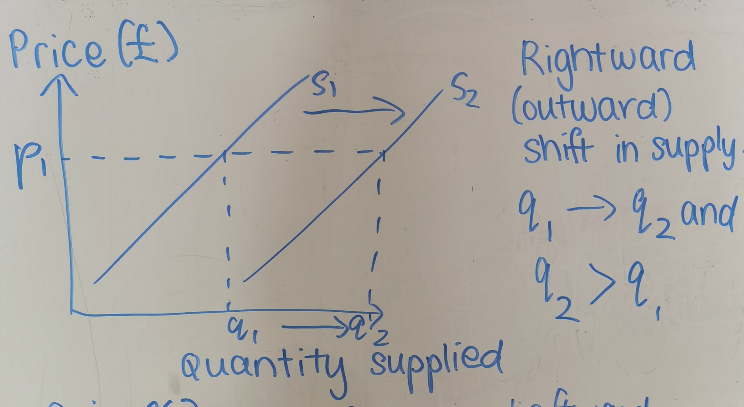
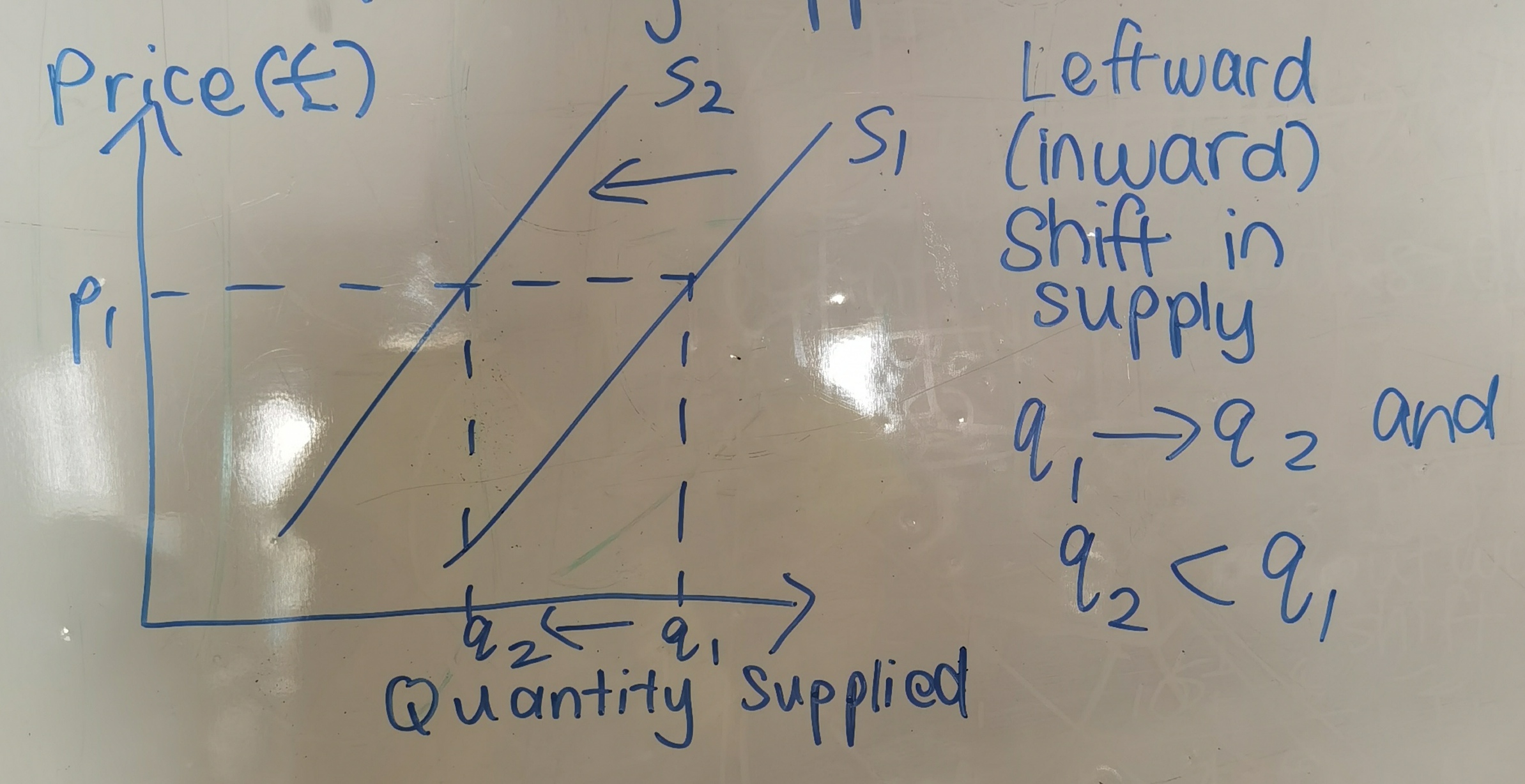
  • == = Graph showing how much of a good will be supplied by producers at different prices.==Positive slope== → Goes up from left to right →==Proportional relationship**== for price & amount demanded:↑ price → ↑ quantity supplied (more profit incentive)↓ price → ↓ quantity supplied (less profit incentive)==Change in price of originally-investigated good== → Movement along supply curve.==Factors NOT related to a change in price of the originally-investigated good
  • \

  

• == → Shift in supply curve.==Rightward/outward supply shift== → ↑ supply==Leftward/inward supply shift== → ↓ supplyPrice is ALWAYS on==y-axis.==Quantity supplied is ALWAYS on

• \

• \

1. \

2. \

3. \

4. \

5. \

6. \

7. \

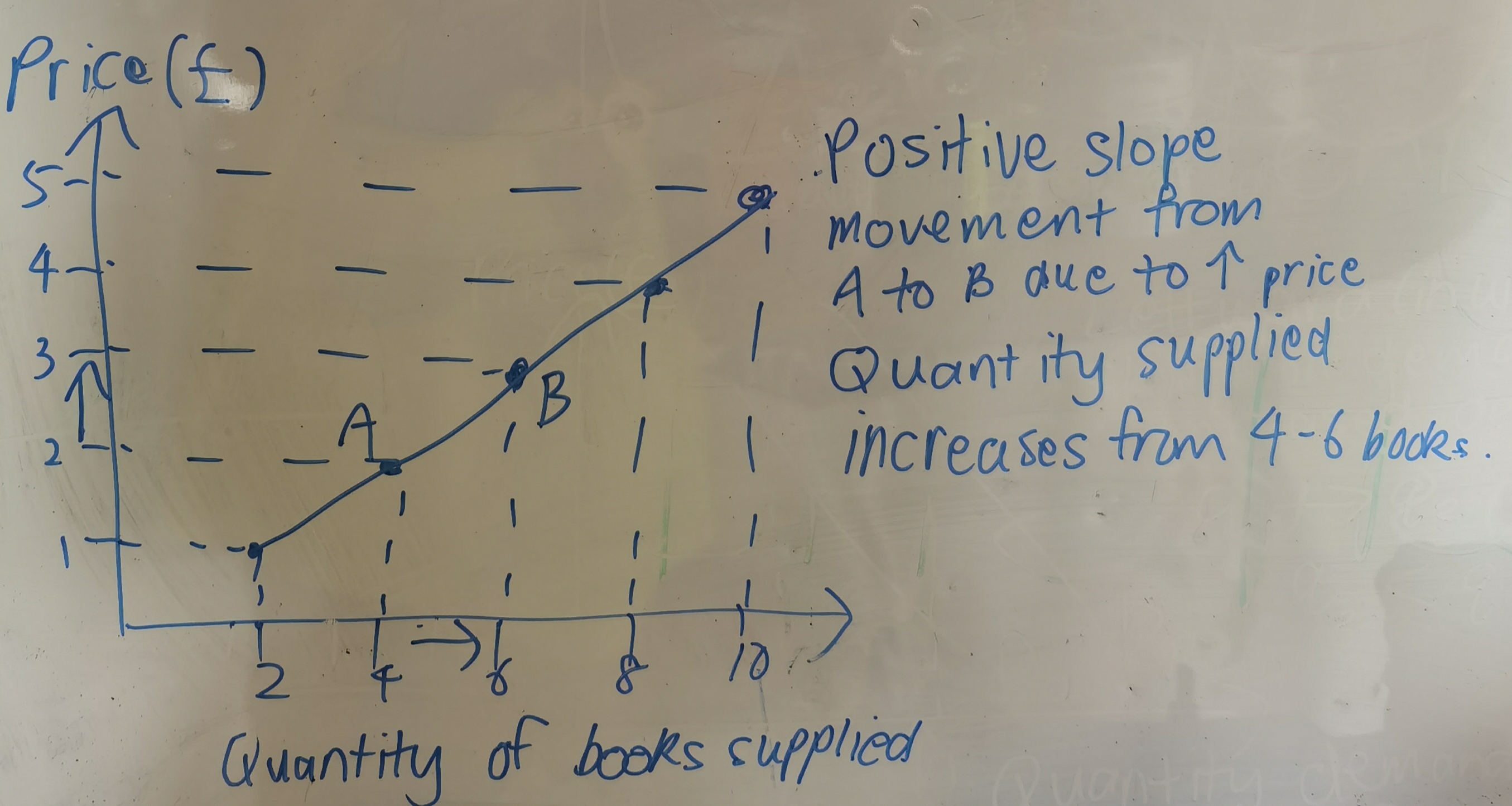
8. ==**x-axis.**Example:==Supply schedule* = Table of the quantity supplied of a good at different price levels, used to calculate expected quantity supplied and plot points on supply curve.Example:Price (£) of BooksQuantity of books supplied12243648510==Fixed supply*== = Supply stays the same regardless of price because it is impossible to increase supply even when price increases, due to a fixed quota.E.g. the number of tickets to seats in a stadium, as the capacity is constant.Factors causing Shifts in the Supply Curve - Syllabus 1.1.3(f)Use==PINNS== acronym:==Production cost - Inversely proportional to supply==Production cost = Price of producing a good/service.e.g. machinery costs (capital), wages (labour), raw materials (land).↑Production cost → ↓ Supply (Less profit incentive)↓Production cost → ↑ Supply (More profit incentive)

   1. \
   2. \

9. \

   10. \

   11. \

   12. \

   13. \

   14. ==Indirect taxes - Inversely proportional to supply==Direct tax = Tax levied on the tax payer’s income or profits.

   15. \

   16. \

   17. ==Indirect tax== = Tax levied on spending than directly on the tax-payer’s income/profits.E.g.: **==VAT==**= Value Added Tax, tax put on goods/services.Used to discourage consumption of harmful or unenvironmental products (e.g. cigarettes, alcoholic beverages) and raise revenue for government expenditure.↑Indirect tax → ↑Production cost → ↓Supply (less profit incentive)↓Indirect tax → ↓Production cost → ↑Supply (more profit incentive)==New technology - Directly proportional to supply==↑New technology → ↑Supply (New technology can be more efficient/productive, and lower production costs as machinery can replace labour, reducing costs from wages.)↓New technology → ↓Supply

   18. \

   19. \

   20. \

• ==Natural factors==Natural disasters, pests, diseases, and bad weather → ↓Supply of agricultural goods/services.Good growing conditions and weather → ↑Supply for agricultural goods/services==Subsidies - Directly proportional to supplySubsidies
• \
• \
• \
• 

• \

• 

• 

• \

  

• \

• 

• \

• 

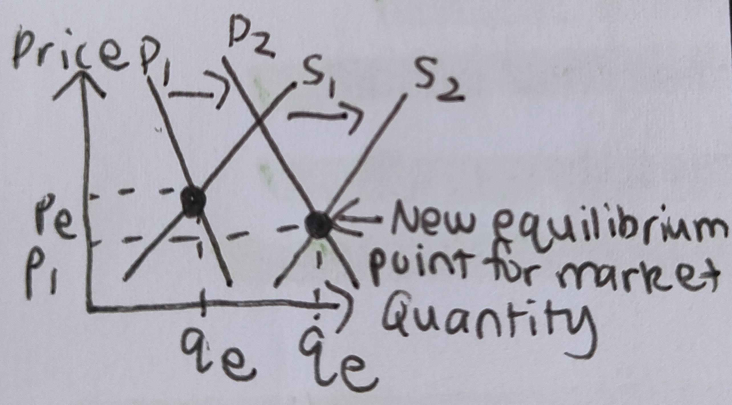
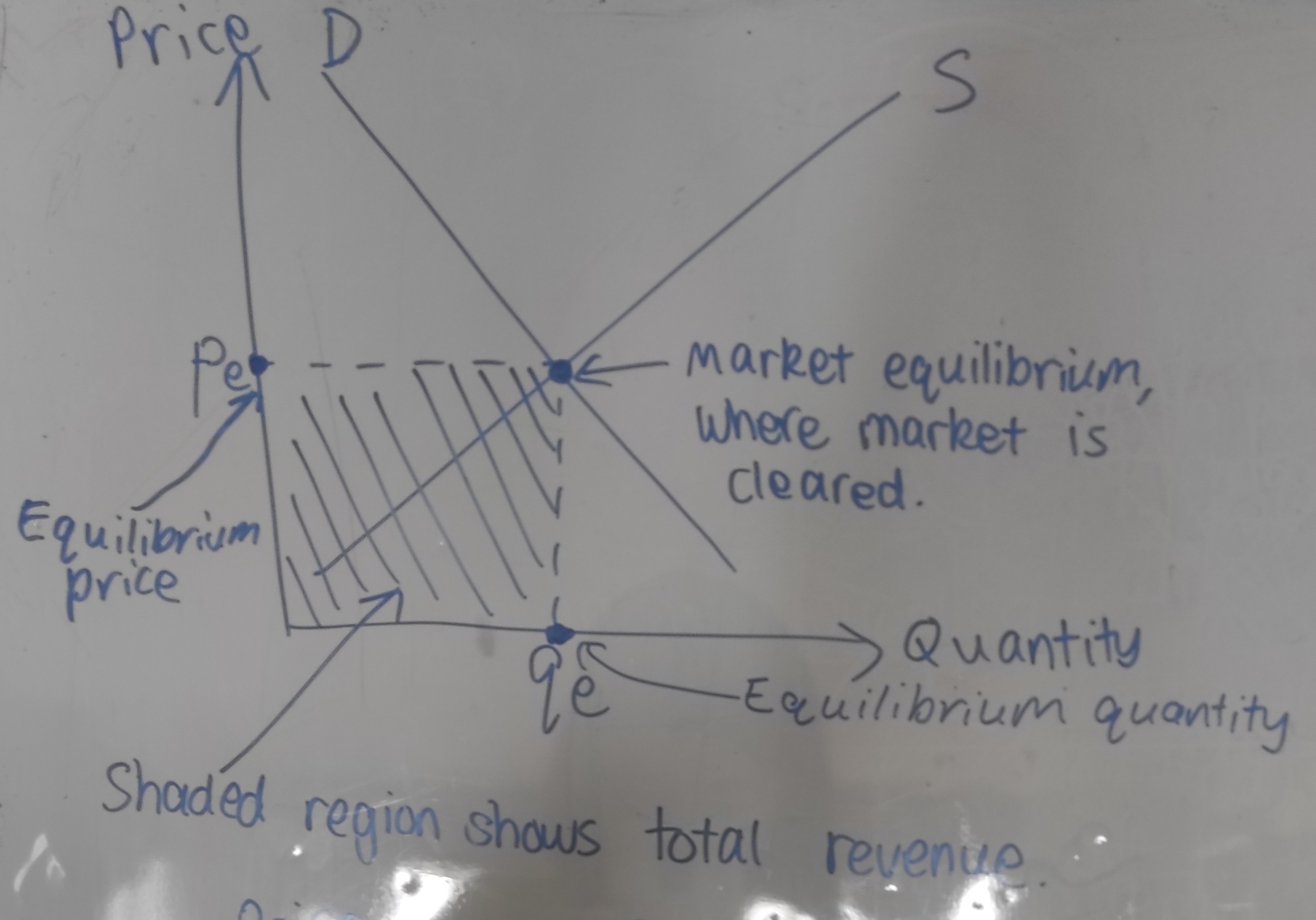
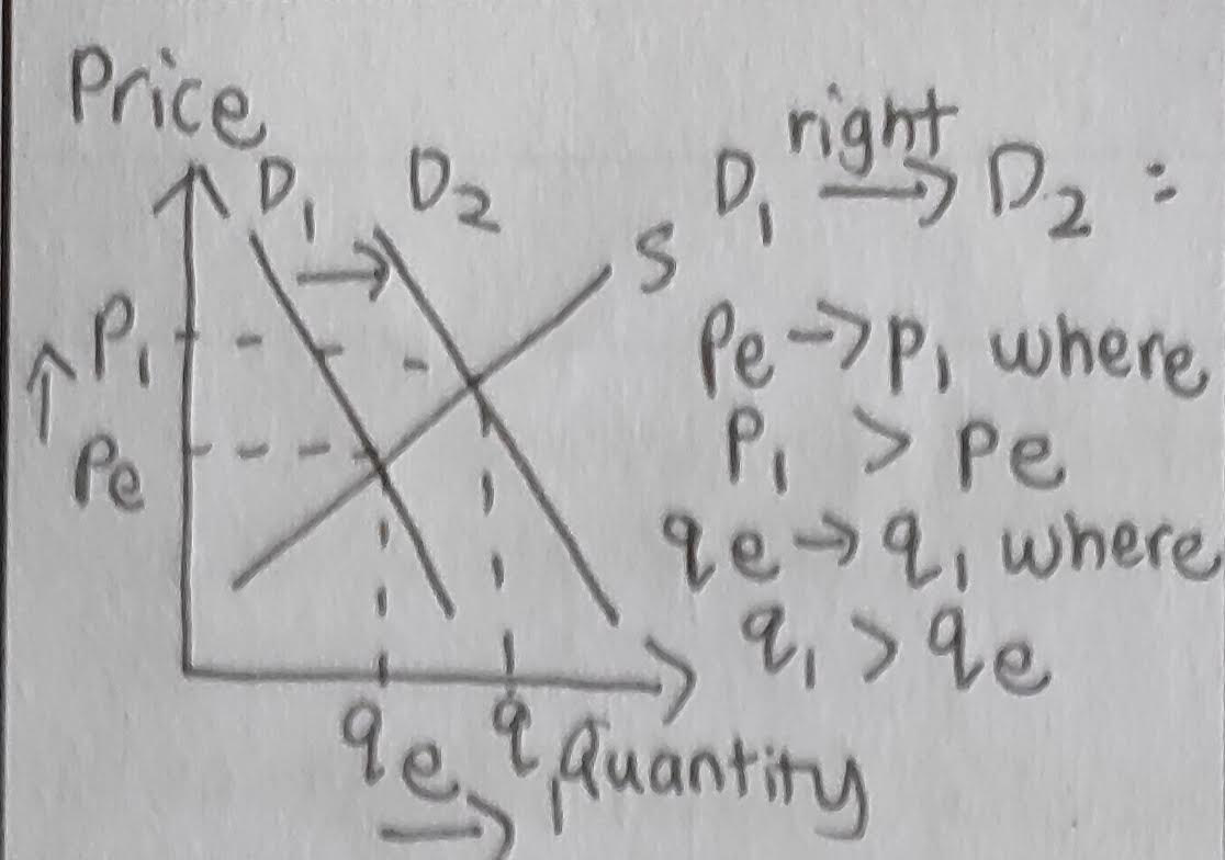
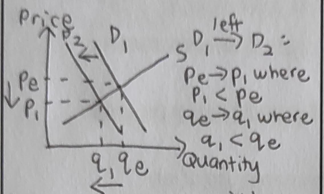
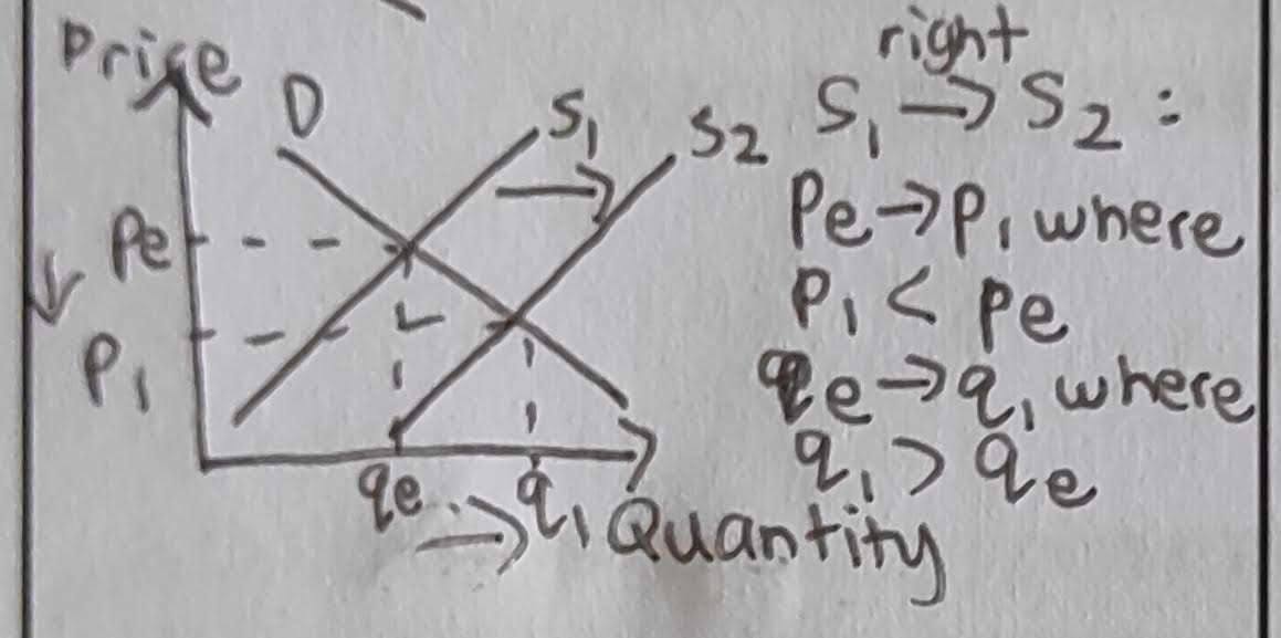
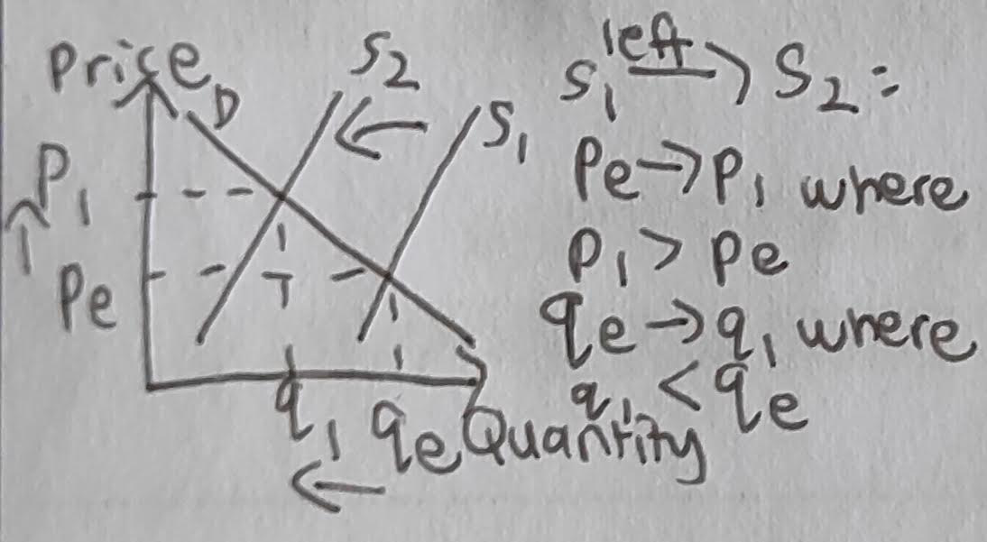
• == = Money paid by government/organization to encourage production of a good/service.↑Subsidies → ↓Production cost → ↑Supply↓Subsidies → ↑Production cost → ↓SupplyEquilibrium Price and Quantity - Syllabus 1.1.3(g)==**Equilibrium price (Market clearing price)****== = Price where the quantity supplied = quantity demanded.Price at intersection of demand and supply curve for the same product.==Cleared market== = Amount supplied in market is completely bought by all consumers; no buyers left without goods, no sellers left with unsold stock.==**Equilibrium quantity***== = Quantity of a good supplied in the market which is equal to demanded quantity.Quantity at intersection of demand and supply curve for the same product.==Total revenue== = Total money earned from selling goods/services = Price/unit * Quantity of units.Market Equilibrium Diagrams - Syllabus 1.1.3(h)==Right demand shift== → ↑Equilibrium price & ↑Equilibrium quantity==Left demand shift== → ↓Equilibrium price & ↓Equilibrium quantity==Right supply shift== → ↓Equilibrium price & ↑Equilibrium quantity==Left supply shift== → ↑Equilibrium price & ↓Equilibrium quantityDemand and supply curves can shift==simultaneously==.Defining, drawing, and calculating excess demand and excess supply - Syllabus 1.1.3(i)

  

• \

  

• \
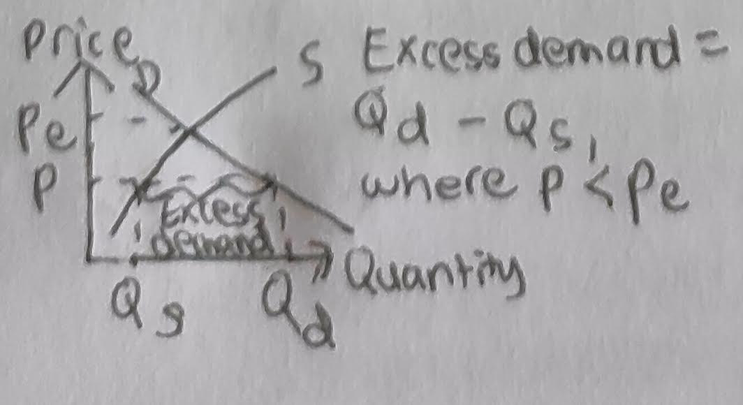
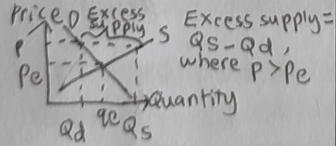
• ==Excess demand**== = Quantity demanded - Quantity suppliedQuantity demanded > Quantity supplied → Supply shortages → Consumers left without goods.Happens when price < equilibrium price.==Excess supply**== = Quantity supplied - Quantity demandedQuantity supplied > Quantity demanded → Demand shortages → Producers left with unsold goods.Happens when price > equilibrium price.Restoring Market Equilibrium - Syllabus 1.1.3(j)==Market disequilibrium
• == = When quantity supplied ≠ quantity demanded.==Removing excess demand**==:Raise selling price from below equilibrium to equilibrium. (↑Price → ↓Demand)Use more resources and shift supply right to satisfy demand.