Descriptive statistics pt1
Descriptive Statistics
Definition: a set of techniques for summarizing and displaying data.
Measurement Scales
Descriptive statistics vary based on measurement scale:
Categorical: Mean, Mode, Median not applicable.
Ordinal: Median, Mode applicable.
Interval/ratio: Mean, Median, Mode applicable.
→ Measuring a variable refers to the act of assigning a value/level of a variable to an individual
→ Calculating frequencies refers to the act of counting how many individuals are characterized by each value/level of the variable NB frequencies can be calculated only after a variable has been measured
Key Features of Variables
Shape of the Distribution
Central Tendency
Dispersion (Variability)
Central Tendency
Measures: Mean, Median, Mode.
Mean: Average, affected by extreme values.
Median: Middle value, less affected by skewness
Mode: Most frequent value, applicable to any type of data
Dispersion
Measures: Range, Interquartile range, Standard deviation, Variance.
Range: Difference between maximum and minimum.
Interquartile Range (IQR): 75th - 25th percentile.
Standard Deviation: Average distance from the mean.
Distribution Shape
Distribution = generic term that refers to how the frequencies are distributed across all the possible values/levels of a variable
Can be represented by:
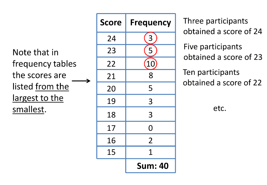
Frequency Tables: List of observed frequencies of each value → frequency indicates the number of people in the sample/population, characterized by that value of the variable - NB note that counting the frequency associated to each level (or value)
of a variable is not the same as measuring the variable
Frequency tables can also be used fro categorical variables → in this case tho they cannot be used to evaluate the shape of the distribution NB although the concept of frequency applies to categorical variables, the concept of shape of the distribution does not
JASP: “Descriptives” icon → “Descriptive Statistics” → Select from the left window the appropriate variable, and drag it to the right window → flag the “Transpose descriptive statistics” → Then we select the Tables menu and we flag the Frequency tables option → Now let’s try to obtain combined frequency tables
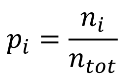
Probability: for a set of emprirical observations, the probability pi of observing the value i of a variable is given by the number ni of observations of the i value, divided by the total number of observations ntot
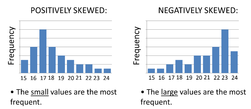
Histograms: Graphical representation of the distribution of variables - conceptually the same as frequency tables
→ JASP:
Shape classifications: unimodal (when the histogram corresponding to the distribution of a quantitative variable shows one single peak), bimodal (two peaks), symmetric, positively skewed, negatively skewed.
Normal Distribution
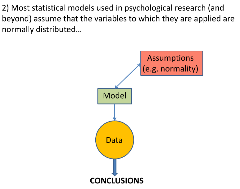
Characteristics: Unimodal, symmetric.
Importance: Many statistical methods assume normality.
Normality Testing
Approaches: Visual/graphical tests, Numerical tests, Statistical tests (e.g., Shapiro-Wilk).
Purpose: Determine if variable distribution deviates from normality.
Practical Application in JASP
Generating frequency tables and histograms for data visualization.
Conducting normality tests and interpreting central tendency and dispersion statistics.
NB one serious limitation of JASP is that you can split for only one variable at a time.