Topic 4
Linear Regression
Category and Continuous Variables as Predictors in Regression
moderation: the association between 2 variables is dependent on the status of a 3rd variable
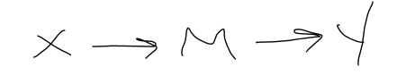
mediation: concerns causal chains
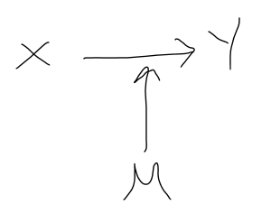
moderation: the relationship between X and Y depends on M
there are 2 main types of variables in regression:
outcome: always continuous in regression
predictor: can be continuous or categorical
the correlation bewteen a categorical predictor and the outcome is the point biserial correlation
categorical variables may include:
individual attributes: membership in one level excludes membership from the others
e.g., gender; male, female
censored variables: artificially created groups
e.g., depression, no depression
categorical predictors with 2 levels can be made artificially quantitative
each level is assigned a numerical code
this code is decided on by the researcher
interpretation of the analysis depends on this coding
one method of doing this is dummy coding
one level = 0, the other = 1
0 = the reference group
1 = the comparison group
depending on which level = 0 and =1, the direction of the correlation will change but the magnitude will not
just need to be aware of this when interpreting results
Additive / Independent / Unconditional Effects of Predictor Variables
This is an example of an additive effect: both predictors contribute directly to the outcome
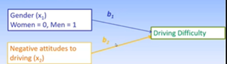
uses the standard regression equation: Y = b0 + b1(x1) + b2(x2) …
recall:
b0 / the constant: what the outcome equals when all predictors = 0
b1 / the slope: the rate of change for the outcome when the given predictor increases by one unit, holding all other predictors constant
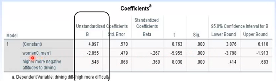
for dummy coded variables, we should be able to tell which level of the predictor produces higher scores on the outcome based on the slope for that variable
interpreting graphs:
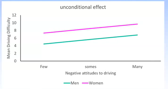
parallel lines indicate the effects of the predictors are additive, and therefore there is no moderator
additive = unconditional = independent effects: the influence of each predictor adds to the explanation of the outcome
Moderated Regression
The Relationship Between Predictors and Outcome Variables at Different Levels of a Third Variable
Example:
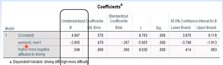
we can plug these values into the regression equation to investigate the effects of driving attitudes on self-regulation for men and women separately:
Y = b0 + b1(X1) + b2(X2)
Women = 0
Low driving attitudes (4): Y = 4.997 – 2.855(0) + .548(4) = 7.33
Moderate driving attitudes (6): Y = 4.997 – 2.855(0) + .548(6) = 8.50
High driving attitudes (8): Y = 4.997 – 2.855(0) + .548(8) = 9.67
Men = 1
Low driving attitudes (4): Y = 4.997 – 2.855(1) + .548(4) = 4.48
Moderate driving attitudes (6): Y = 4.997 – 2.855(1) + .548(6) = 5.65
High driving attitudes (8): Y = 4.997 – 2.855(1) + .548(8) = 6.82
it is evident from these results that as reports of negatve driving attitudes increase, so does driving self-regulation for both men and women
however, independent of driving attitudes, women self-regulate their driving more than men
Moderator Variables in Regression
moderator effect: the influence of one predictor on the outcome is conditional on the score of a second IV
moderator variable: the IV that influences the relationship between the predictor and outcome
Conditional / Non-Independent / Interaction Effects of Predictor Variables
Here, b0 and b1 are the same for men and women:
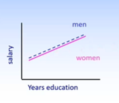
Here, b1 is the same but b0 is different
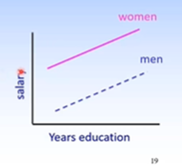
Both of these are examples of independent effects, because the slope is the same
Here, b0 and b1 are different for men and women (2nd graph)
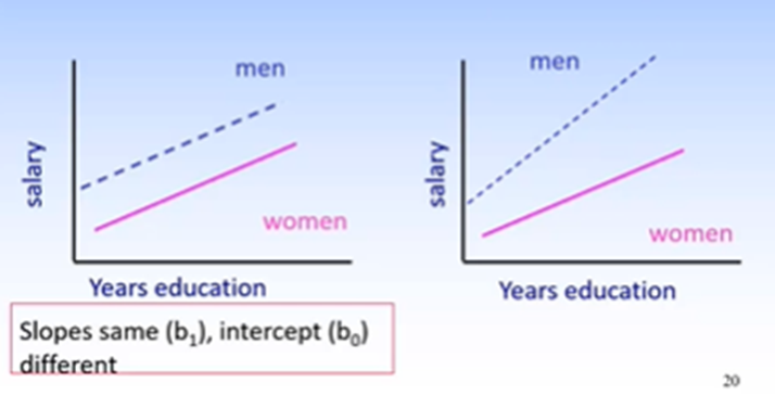
Because the slope is different, the lines are not parallel, and there is a conditional effect present
Interpreting Moderator Coefficients
The equation for a moderated regression analysis contains the moderator term:
Y = b0 + b1(X1) + b2(M) + b3(X1*M)
the moderator term = X*M
B3 indicates: for a 1 unit change in the predictor, the change in score for the outcome is dependent on the score on the moderator
we always use the unstandardise coefficient here, because the unstandardised coefficient for the moderator term cannot be interpreted
we only include b3 if we expect the moderation will be significant
Moderated Regression Analysis with a Category Moderator
example: using IV = driving atitudes, M = gender, DV = driving self-regulation
for men: no sig association between driving attitudes and self-regulation
for women: sig negative association between driving attitudes and self-regulation
need to first check whether the moderator term accounts for a significant proportion of variance in the model - if it does, moderated regression analyses can proceed
Performing a Moderated Regression Analysis
four variables are needed in a moderated regression analysis:
predictor
outcome
moderator
moderator term
we must first confirm the moderator term is significant to conduct a moderated regression analysis
if not, remove it from the analysis and conduct a standard multiple regression
if it is, this means the relationship between the predictor and outcome is conditional on the moderator, so a moderated regression analysis is appropriate
we begin with a hierarchical regression analysis
enter predictor and moderator
enter moderator term
we only report step 1 if the moderator term was nonsignificant
step 1: looks at the linear effect of the predictor and moderator
indicates the effect of the given predictor on the outcome while holding the other IV constant
step 2: looks at the individual effects of the predictor and moderator when they are conditional
indicates the effect of each IV when the other IV and interaction are held constant
these are very different effects and dont make sense to report together
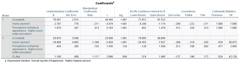
the coefficients table produced doesnt give us a lot of information about how the association between the predictor and outcome differs based on the moderator. there are a few ways to gather this information
using the regression equation
can plug in the values from the coefficients table into the moderated regression equation. for example:
For males:
High perceptions of appearance: ŷ = 83.87 – 16.690(0) + .454(11.852+1.88) + 1.180(0*11.852) = 90.10
Average perceptions of appearance: ŷ = 83.87 – 16.690(0) + .454(11.852) + 1.180(0*11.852) = 89.25
Low perceptions of appearance: ŷ = 83.87 – 16.690(0) + .454(11.852-1.88) + 1.180(0*11.852) = 88.40
For females:
High perceptions of appearance: ŷ = 83.87 – 16.690(1) + .454(11.852+1.88) + 1.180(1*11.852) = 87.40
Average perceptions of appearance: ŷ = 83.87 – 16.690(1) + .454(11.852) + 1.180(1*11.852) = 86.55
Low perceptions of appearance: ŷ = 83.87 – 16.690(1) + .454(11.852-1.88) + 1.180(1*11.852) = 85.69
we get the high/ average/ low perception of appearance values from the frequencies table: use the mean +/- the standard deviation where appropriate
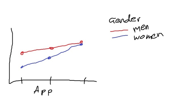
these results, graphically, would look like:
because the lines are not parallel, there is likely a significant moderating effect here
another method is by using simple slopes analysis
Simple Slopes Analysis
simple slopes analyses investigate the association bewteen the predictor and outcome at each level of the moderator variable
for a categorical moderator like gender, we conduct 2 simple slopes analyses; one where women = 0 and men = 1, and one where men = 0 and women = 1
this is because when the reference category is coded 0, the moderator and moderator terms = 0 as well (because anything*0 = 0)
therefore, we can evaluate the association between the predictor and ouctome at both levels of gender
we can do this by splitting the datafile by gender and running the moderated regression again
example:
simple slopes for men:
as p > .05, attitudes to driving did not influence driving self-regulation for men, supporting hypothesis 1
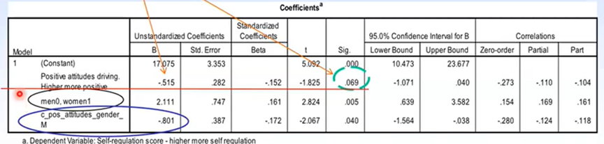
simple slopes for women:
as p < .05, attitudes to driving did influence driving self-regulation for women, supporting hypothesis 2