L3 Descriptive statistics
Revision
Introduction to Variables
Independent Variables: Variables that predict or indicate changes.
Dependent Variables: Variables that are affected by independent variables.
Example Questions:
Effects of tattoos on job interview success.
Impact of scent and music in retail on consumer behavior.
Relation between commutes to work and wages.
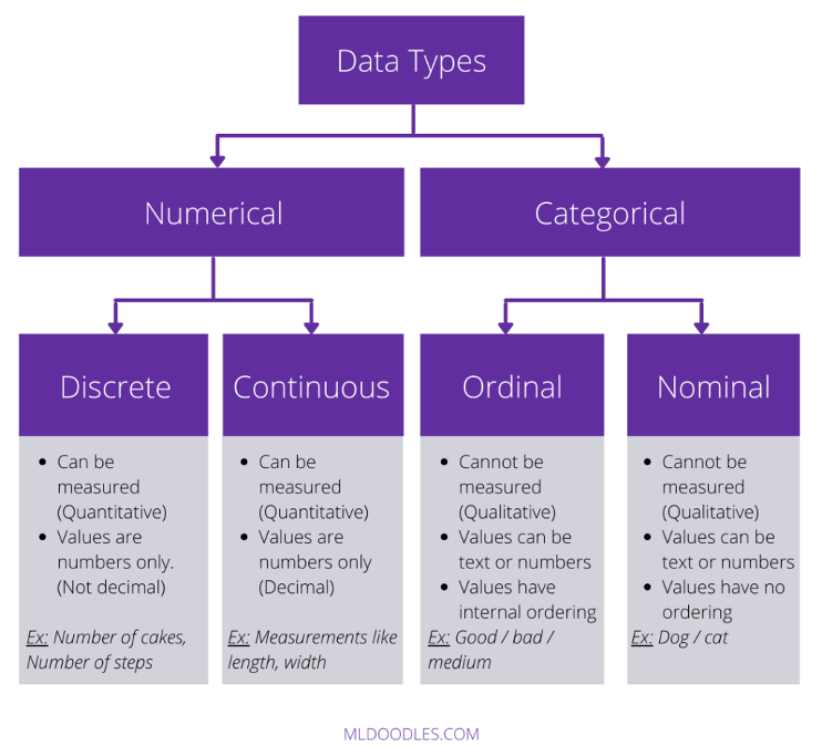
Types of Variables
Nominal Variables: Categorical, non-hierarchical (e.g., colors, types).
Ordinal Variables: Categorical, hierarchical; can rank-order responses (e.g., survey scales).
Scale Variables: Continuous, numerical data with meaningful responses (e.g., temperature, height).
Level of information:
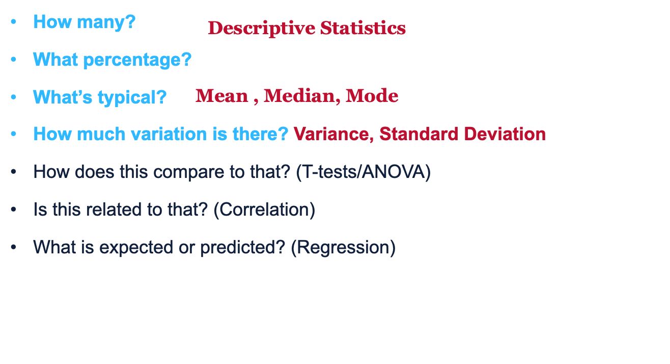
Descriptive Statistics
Descriptive statistics describe and summarize variables one at a time.
Descriptive statistics include measures of central tendency and measures of dispersion.
Descriptive Statistics measures:
Measures of Central Tendency:
Mode: The most frequent value in a dataset.
Median: The middle value when data is sorted.
Mean: The average of all values.
Measures of Dispersion:
Range: Difference between highest and lowest values.
Variance: Measures how much data points differ from the mean.
Standard Deviation: Indicates the average distance of data points from the mean, revealing data spread.
Effects of extreme values on mean vs. median.
Mean/Median/Mode/Range/Dtandard deviation
Relevant to ordinal and scale level variables.
Questions:
Visual Data Representation:
The distribution of variables can be displayed on frequency tables and histograms.
Outliers:
One or more observations that are unusually large or small values (extreme scores).—> Data points that are unlike the rest of the data.
Outliers can be:
ØData incorrectly recorded (data entry error)
ØObservation that doesn’t belong to the population in interest
ØUnusual data value
Methods to identify outliers and review them carefully.
ØSorting data
ØProducing relevant graphs
Outliers remedies:

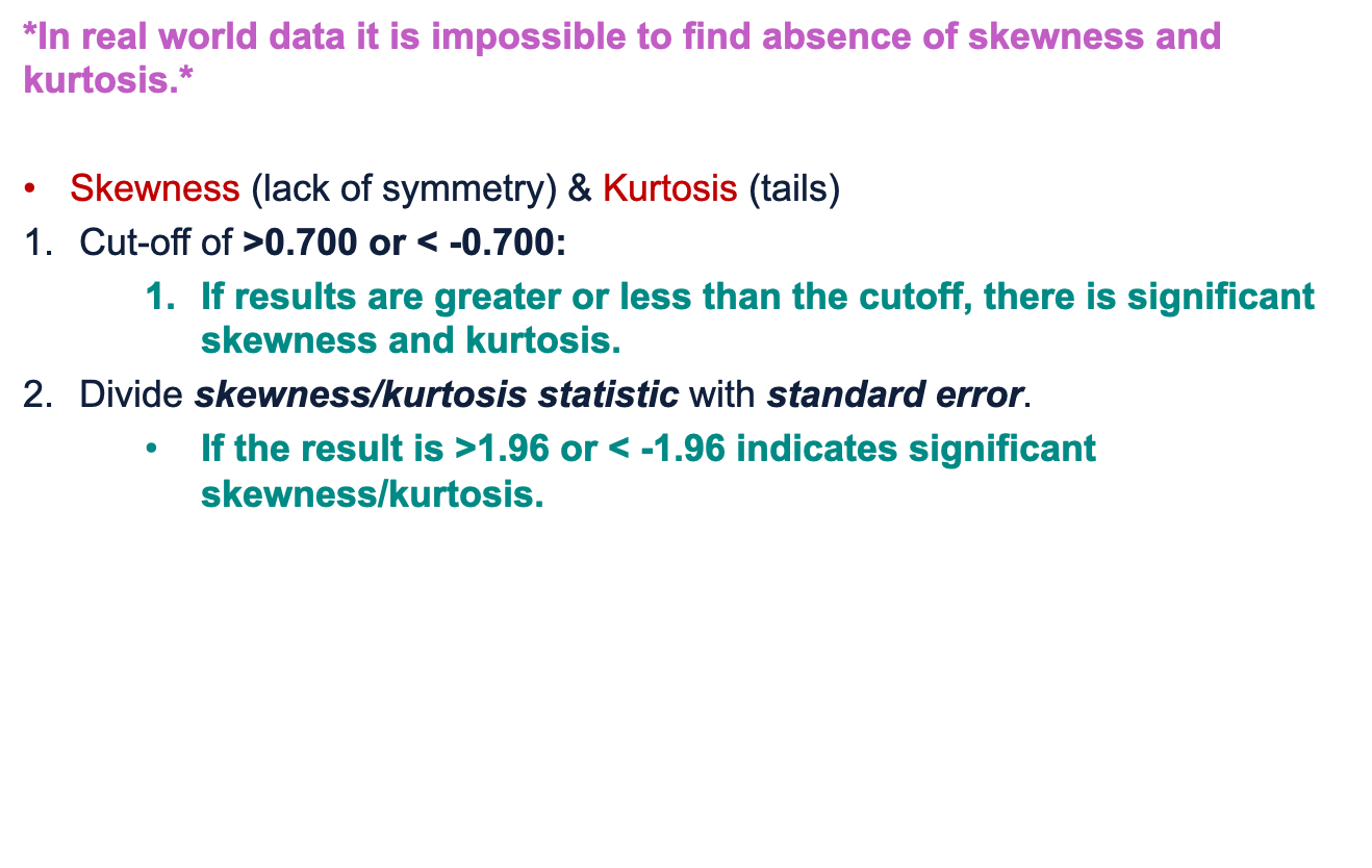
Skewness (asymmetry) and kurtosis (tailedness) of distributions.
Only relevant to ordinal or scale level variables!
Kurtosis refers to the extent to which a set of scores is clustered close to (or far from) the mean.
Whether data is heavy-tailed or light-tailed
Data with high kurtosis have heavy tails and more outliers.
Data with low kurtosis has light tails and fewer outliers.
Skewness measures the asymmetry in the distribution of a variable/data.
Lack of symmetry, data is disproportionally distributed.
Majority of data is clustered in one area and outliers are away from the majority of data.
Shows the direction of outliers
Evaluating kurtosis ans skewness:
Data Cleaning:
Missing values
Respondents skipping questions.
Exact or inexact duplicate values.
Example: Subscribing in a retailer with two different emails.
De-duping – process of removing duplicates
Inconsistencies in the recording of variables.
Example: record student marks raw or in %
Dates, names, phone numbers recorded with inconsistent formats.
Missing data —>
How to identify missing data?
Visual scan (small datasets only).
Count empty cells.
Check against total cases.
Use specific function in each software.
Potential remedial actions:
Discard observations with missing data
Discard variables with missing values
Fill in missing entries with estimated values (imputation)
Apply data mining algorithms that handle missing values.