Matrices
Introduction
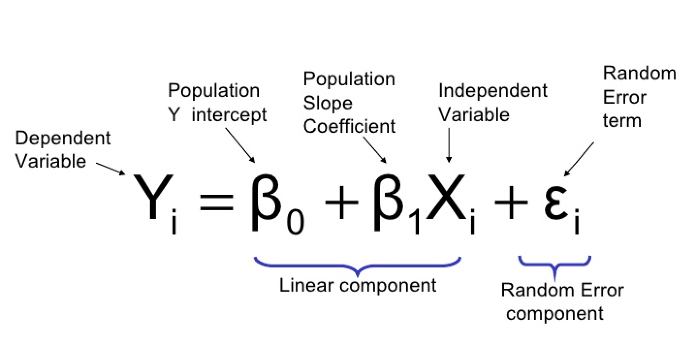
The Linear Model Formula states that the relationship between variables can be expressed in matrix form, allowing for efficient computation and analysis of data sets.
What does it mean?
Y : The thing you're trying to predict (e.g., how much a gene is expressed).
β0: The starting point (the value of Y) when everything else is zero).
β1 : How much Y changes when x_1 changes.
X1 : The factor that might influence Y (e.g., a treatment or condition).
epsilon : A small "oops" factor (random noise or error).
How It Works
Think of it like this:
You’re trying to draw a straight line through some data points.
β0 is where the line starts (the intercept).
β1 x1 tilts the line (the slope).
The formula combines these to make predictions about Y
More Predictors?
If there’s more than one factor, we just add them:
y = β0 + β1 X1 + β2 X2 +…+ ε
Each X is a different factor, and each β shows how much that factor influences Y
A Simple Example
Imagine you’re studying how sunlight X1 affects plant growth Y:
If sunlight increases by 1 hour, the plant grows by 2 cm.
The formula might look like this:
Plant Growth = 5 + 2 x Sunlight + ε
5: The baseline growth without any sunlight.
2: How much growth changes with each extra hour of sunlight.
ε : A bit of randomness (e.g., soil differences).
Questions
Here are the answers to the problems:
Problem 1: Basic Interpretation
Model:
y = 10 + 3x
Crop yield when no fertilizer is used (\(x = 0\)):
y = 10 + 3(0) = 10
Answer: 10 units.
Increase in crop yield for every additional unit of fertilizer:
This is given by the coefficient of \(x\), which is 3.
Answer: 3 units per unit of fertilizer.
Crop yield when \(x = 5\):
\[ y = 10 + 3(5) = 10 + 15 = 25 \]
Answer: 25 units.
Problem 2: Adding Random Error
Model:
y = 8 + 1.5x + ε
Plant height for x = 4 , ε = 0.5):
y = 8 + 1.5(4) + 0.5 = 8 + 6 + 0.5 = 14.5
Answer: 14.5 units.
Plant height for x = 6 , ε = -0.3:
y = 8 + 1.5(6) - 0.3 = 8 + 9 - 0.3 = 16.7
Answer: 16.7 units.
Problem 3: Multiple Predictors
Model:
y = 5 + 2x_1 + 3x_2
Predict y when X1 = 10, x2 = 20:
y = 5 + 2(10) + 3(20) = 5 + 20 + 60 = 85
Answer: 85 units.
Effect of increasing X1 by 1 while X2 stays the same:
The coefficient of X1 is 2, so Y increases by 2.
Answer: Increase of 2 units.
Baseline growth Y when x1 = 0 and X2 = 0:
y = 5 + 2(0) + 3(0) = 5
Answer: 5 units.
Problem 4: Real-Life Scenario
Model:
y = 50 + 4x_1 - 2x_2 + ε
If x_1 = 2, x_2 = 10, ε= 1:
y = 50 + 4(2) - 2(10) + 1 = 50 + 8 - 20 + 1 = 39
Answer: 39 units.
Effect of increasing treatment X1 by 1 unit:
The coefficient of X1 is 4, so Y increases by 4.
Answer: Increase of 4 units.
Effect of increasing age X2 by 1 unit:
The coefficient of X2 is -2, so Y decreases by 2.
Answer: Decrease of 2 units.
Problem 5: Visual Understanding
Model:
y = 40 + 5x
Plot the line for x = 0 to x = 10:
Key points:
x = 0, y = 40 + 5(0) = 40
x = 10, y = 40 + 5(10) = 90\)
Plot these points and draw a straight line.
Intercept Y when x = 0:
y = 40
Answer: 40.
Slope 5 and its meaning:
The slope indicates that Y increases by 5 for every 1 unit increase in X (study hours).
Answer: Y increases by 5 for every additional hour of study.
Let me know if you'd like further clarification!
Residual sum of squares
**What is the Residual Sum of Squares (RSS)?**

---

When we create a linear model, we want the line (or hyperplane) to be as close as possible to the actual data points.

- Each data point has an **actual value** (\\( y_i \\)) and a **predicted value** (\\( \\hat{y}_i \\)) based on the model.
- The **difference** between the actual and predicted value is called the **residual**:
\\[
\\text{Residual} = y_i - \\hat{y}_i
\\]
- The **Residual Sum of Squares (RSS)** is just the sum of the squares of all these residuals:
\\[
\\text{RSS} = \\sum_{i=1}^n (y_i - \\hat{y}_i)^2
\\]

---

### **Why Do We Care About RSS?**

- The RSS tells us how far off our model's predictions are from the actual data.
- **Goal**: We want the RSS to be as small as possible. A smaller RSS means the model fits the data better.

---

### **How Does RSS Help Estimate \\(\\beta\\)?**

In a linear model:
\\[
\\hat{y}*i = \\beta_0 + \\beta_1 x*{1i} + \\beta_2 x_{2i} + \\dots
\\]

The predicted value (\\( \\hat{y}_i \\)) depends on the \\(\\beta\\) coefficients, which are the weights of the predictors.

To find the best \\(\\beta\\) values:

1. **Minimize the RSS**:
    - The best \\(\\beta\\) values are those that make the RSS as small as possible.
    - This process is called **least squares regression**.
2. **Optimization**:
    - Mathematically, we minimize:
    \\[
    \\text{RSS} = \\sum_{i=1}^n (y_i - (\\beta_0 + \\beta_1 x_{1i} + \\beta_2 x_{2i} + \\dots))^2
    \\]
    - By solving this minimization problem (using calculus or linear algebra), we calculate the \\(\\beta\\) coefficients.

---

### **Simple Example**

Imagine we have one predictor \\( x \\) and are modeling \\( y = \\beta_0 + \\beta_1 x \\).

### Steps to Estimate \\(\\beta_0\\) and \\(\\beta_1\\):

1. **Write the RSS**:
\\[
\\text{RSS} = \\sum_{i=1}^n (y_i - (\\beta_0 + \\beta_1 x_i))^2
\\]
2. **Find \\(\\beta_0\\) and \\(\\beta_1\\) that minimize RSS**:
    - Take derivatives of RSS with respect to \\(\\beta_0\\) and \\(\\beta_1\\).
    - Set the derivatives to 0 to solve for the \\(\\beta\\) values.
3. **Solution**:
Using formulas derived from this process:
    - \\(\\beta_1 = \\frac{\\text{Cov}(x, y)}{\\text{Var}(x)}\\) (slope).
    - \\(\\beta_0 = \\bar{y} - \\beta_1 \\bar{x}\\) (intercept).

---

### **Key Takeaway**

- The RSS is the function we minimize to find the best \\(\\beta\\) coefficients in a linear model.
- By minimizing the RSS, we ensure the model fits the data as closely as possible.

Does this help clarify? Let me know if you’d like to see a worked-out numerical example!
Matrix notation
Matrix operations