Microeconomics synthesis flashcards
Microeconomics synthesis
Chapter 1
Intro
Microeconomics: the study of the allocation of scarce resources
Microeconomics is all about dealing with limited resources. It's like a game of choices where people, businesses, and governments have to decide what goods and services to produce , how to make it, and who gets it because we can't have everything we want (Trade Offs)
Ex: if a company makes more cars, it means they have to make fewer other things, like bicycles or computers because they only have a limited amount of resources like workers, materials, and money.
These decisions can be made by the government or by individuals and businesses making choices. Prices play a critical role in determining what is produced, how it's produced, and who gets it. Interactions in markets between buyers and sellers help set these prices.
EX: If something is expensive, not many people can buy it, but if it's cheap, more people can.
1.1 Model
Economists use models to understand these relationships and make predictions predictions and understand cause-and-effect relationships. They help explain resource allocation and the impact of price changes on consumer behavior and production. So, like a map that helps them figure out how changes in one thing, like price, will affect something else, like how much of a product gets made.
Making assumptions is necessary to create manageable models.
Constraints :
Desire (unlimited) → means (limited) so we have to make choices.
Consumers: the objective is having a maximum well being, the constrains are prices, income (limitation on spending power)
Producers: Their objective is a maximum profit, their constraints are demand-technology
Government: Decides which goods + services to produce and how to regulate w/ taxes. Their constraints are imposed by limited resources + the behavior of consumers and firms.
Testing Theories: Economists test theories through the prediction of cause-and-effect relationships. They use models to make clear, testable predictions. If predictions don't align with reality, the theory may be rejected.
Positive vs. Normative Statements: Positive statements are testable hypotheses about cause and effect they can be tested , while normative statements express value judgments or opinions about what should happen sot hey can’t be tested
Positive statement: a testable hypothesis about cause and effect
Normative statement: a CCL as to whether something is good or bad.
Uses of microeconomic models
Microeconomics explain why eco decisions are made and allow us to make predictions, they are useful for individuals, gov and firms in making decisions .
Individuals 🡪 Can use models for purchasing decisions, to make choices on what to buy considering factors like price, personal preferences etc.
Firms 🡪 Production methods: they use it to determine the most cost-effective production methods …
Government: they use it to predict the effects of proposed policies before implementing them
Chapter 2
The supply-and-demand model describes how consumers and suppliers interact to determine the quantity and price of a good or service. It provides a good description of how competitive markets function (it allows us to make accurate predictions easily.)
To use the model, you need to determine three things:
Buyers’ behavior
Sellers’ behavior
How they interact.
2.1. Demand
Potential consumers decide how much of a good or service to buy based on its price and many other factors, including :
Consumers’ tastes determine what they buy. Consumers do not purchase foods they dislike or clothes they view as unfashionable or uncomfortable. Advertising may influence people’s tastes.
Information (or misinformation)about the characteristics of a good affects consumers’ decisions.
EX: if consumers are convinced that oatmeal could lower their cholesterol level, they would rush to grocery stores and buy large quantities of it.
The prices of other goods also affect consumers’ purchase decisions:
The price of a close substitute: a product that you view as similar or identical to the one you are considering purchasing is much lower than the price of Levi’s jeans, you may buy that brand instead.
The price of a complement: a good that you like to consume at the same time as the product you are considering buying can affect your decision.
Ex: If you eat pie only with ice cream, the higher the price of ice cream is, the less likely you are to buy pie.
Income: plays a major role in determining what and how much to purchase. If you have a large amount of money, you will purchase more.
Government rules and regulations affect purchase decisions.
Sales taxes increase the price that a consumer must pay for a good,and government-imposed limits on the use of a good may affect demand. Ex: When a city’s government bans the use of skateboards on its streets, skateboard sales fall.
Other factors; ex: trends
Economists usually concentrate on how price affects the quantity demanded1.
The relationship between price and quantity demanded plays a critical role in determining the market price and quantity in a supply-and-demand analysis. To determine these changes economists must be careful of other factors that affect demand, such as income and tastes.
The Demand Curve
DEF: The quantity demanded is the amount of a good that consumers are willing to buy at a given price, holding constant other factors that influence purchases
The quantity demanded of a good or service can exceed the quantity sold.
EX: as a promotion, a local store might sell dark chocolate bars for $1 each today only. At that low price, you might want to buy 10 chocolate bars, but because the store has only 5 remaining, you can buy at most 5 chocolate bars at this price. The quantity you demand at this price is 10 chocolate bars—it’s the amount you want—even though the amount you can buy is only 5.
A demand curve shows the quantity demanded at each possible price, holding constant other factors that influence purchases.
In a supply and demand graph, the vertical axis of the graph measures the price, p, per unit of the good. Here, we measure the price of coffee in dollars per pound (“lb”). The horizontal axis measures the quantity, Q,of the good in a physical measure per period. Here, we measure the quantity of coffee demanded in millions of tons per year.
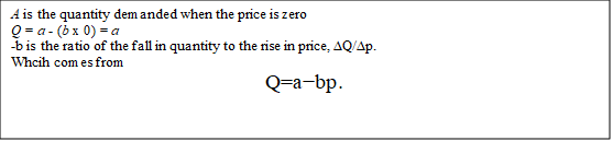
The demand curve hits the vertical axis at $12, indicating that the quantity demanded is zero when the price is $12 per lb or higher. The demand curve hits the horizontal quantity axis at 12 million tons per year, which is the quantity of coffee that consumers would want if the price were zero.
The demand curve only shows how quantity varies with pricebut not how quantity varies with other variables. The demand curve answers the question “What happens to the quantity demanded as the price changes when all other factors are held constant?”
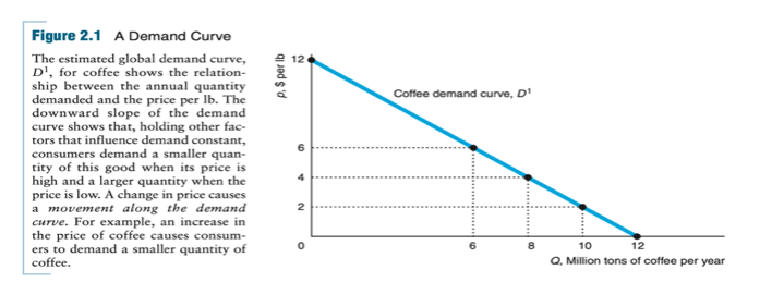
The Law of Demand: Consumers demand more of a good if its price is lower, holding constant other factors that influence the amount they consume. So, the demand curve has a down-forward slope.

Movement along the demand curve: it’s when the price of good changes and people buy more or less of a product because of it, assuming that everything else, like their income or preferences, stays the same. (The quantity demanded changed because the price changed.)
If the price goes down, they usually buy more (expansion along the demand curve).
If the price goes up, they usually buy less (contraction along the demand curve).
 The demand curve is like a map that shows how much people want to buy at different prices, and moving along it shows how price changes affect how much people buy.

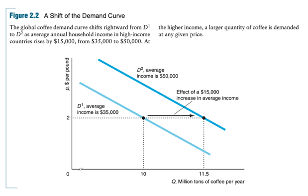
A change in any factor other than the price of the good itself results in a shift of the demand curve.
A change in other factors, such as the prices of substitutes and complements, may also cause a demand curve to shift.
Substitute: a good or service that may be consumed instead of another good or service.
Ex:Tea is a substitute for coffee, so a decrease in the price of tea may cause their demand curve to shift to the left. (Since people would be more attracted to buy tea since it is cheaper)
Complement: a good or service that is jointly consumed with another good or service.
Ex: many people drink coffee with sugar. An increase in the price of sugar would cause their demand curves to shift to the left.
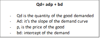
The Demand Function
The demand function shows the effect of all the relevant factors on the quantity demanded.
The Case, (mise en condition): We examine a demand function for coffee.
Q is the quantity of coffee demanded, which varies with the price of coffeep, the price of sugar, ps, and consumers’ income, Y, so the coffee demand function, D
In general;
Q = D(p, ps, Y).
Q is the quantity of the good demanded
p, is the price of the good
Autre facon de faire si on te donne un tableau avec des donners:
Price | Quantity demanded |
0,5 | 500 |
1 | 400 |
1,5 | 300 |
2 | 200 |
2,5 | 100 |
Ex:
1st step : To find the slope do : ∆Q/∆P
ad= = -200 Qd= -200p + bd
2nd step : find the intercept demanded 🡪 You can do so by plunging any row
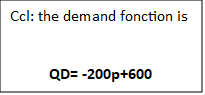 Ex: 200= -200.2 + bd
200=-400+bd
200+400=bd
Db = 600
2.2. Supply
We also need to know how much firms want to supply at any given price. Firms determine how much of a good to supply based on the price of that good and other factors such as:
The costs of productionaffect how much firms want to sell a good. As a firm’s is cost falls, it is willing to supply more. (si les couts de production sont bas les producteurs vont plus offrir). If the firm’s cost exceeds what it can earn from selling the good, the firm sells nothing. (si les facteurs de production sont hauts les producteurs vont offir peux). Thus, factors that affect costs also affect supply.
Government rules and regulationsaffect how much firms want to sell or whether they may sell a product. Taxes and many government regulations such as those covering pollution, sanitation, and health insurance alter the cost of production.
The Supply Curve
The quantity supplied is the amount of a good that firms want to sell at a given price, holding constant other factors that influence firms’ supply decisions, such as costs and government actions.
It shows the quantity supplied at each possible price, holding constant the other factors that influence firms’ supply decisions.
The supply curve answers the question “What happens to the quantity supplied as the price changes, holding all other factors constant?”
Effects of Price on Supply:
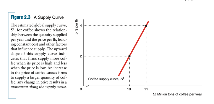
The supply curve is upward-sloping. As the price increases, firms supply more. (If the price is $2 per lb, the quantity supplied by the market is 10 million tons per year. If the price rises to $4, the quantity supplied rises to 11 million tons.)

An increase in the price of coffee causes a movement along the supply curve —> firms supply more coffee.
Compared to the “Law of Demand” there is no “Law of Supply” that requires the market supply curve to have a particular slope.
The market supply curve can be upward-sloping, vertical, horizontal, or downward-sloping. Along such supply curves, the higher the price, the more firms are willing to sell, holding costs and government regulations fixed.
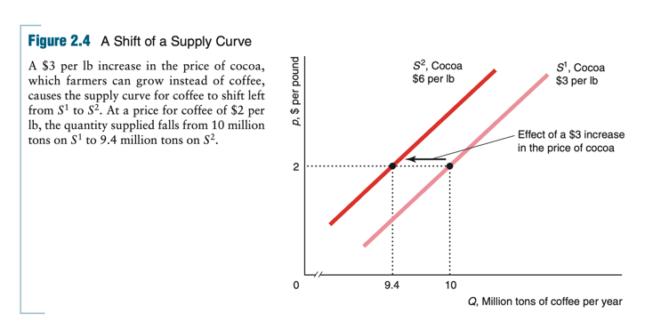 Effects of Other Variables on Supply: A change in a factor other than a product’s price causes a shift of the supply curve.
EX: Suppose the price of cocoa (which is a key input in making chocolate) increases from $3 to $6 per lb. The land on which coffee is grown is also suitable to grow cocoa. When the price of cocoa rises, some coffee farmers switch to producing cocoa. Therefore, when the price of cocoa rises, the amount of coffee produced at any given coffee price falls. (When cocoa prices go up, farmers who grow both coffee and cocoa prefer to grow more cocoa because it's more profitable. So, they reduce coffee production to grow more cocoa, causing less coffee to be available, even if coffee prices stay the same)

Reminder: When the coffee price changes, the change in the quantity supplied reflects a movement along the supply curve. When costs, government rules, or other variables that affect supply change, the entire supply curve shifts.
 The Supply Function
The supply function shows the relationship between the quantity supplied, price, and other factors that influence the number of units offered for sale.
The coffee supply function i
Q = S(p, pc )
Q is the quantity of coffee supplied
p is the price of the coffee
pc is the price of cocoa.
Autre facon de faire si on te donne un tableau avec des donners: (same as the demand)
Summing Supply Curves
The total supply curve shows the total quantity produced by all suppliers at each possible price.
Summing up individual supply curves to create a market supply curve involves adding together the quantities that each producer is willing to supply at different prices.
 Individual Suppliers: Think of various suppliers or sellers, like farmers, companies, or individuals, each with their own supply curve. These curves show how much of a product they're willing to sell at different prices.
Combine Quantities: To create a market supply curve, you add up the quantities that each seller is willing to supply at each price. So, at a specific price, you add how much each supplier is willing to sell.
Market Supply Curve: This combination of quantities at different prices gives you the market supply curve. It shows how much of the product is available in the entire market at various prices.
Shifts and Changes: Just like individual supply curves, the market supply curve can shift left or right due to changes like more suppliers entering the market or improvements in production methods. These shifts affect the total supply in the market.
Finding Equilibrium: The point where the market supply curve meets the demand curve (representing what buyers want) is the equilibrium. It's where the price and quantity satisfy both buyers and sellers.
Summing up supply curves helps us understand how the total supply in a market changes with different prices and other factors. It's crucial for understanding how markets work and reach a balance between what's supplied and what's demanded.
How Government Import Policies Affect Supply Curves
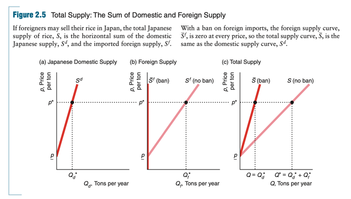
We can use this approach for deriving the total supply curve to analyze the effect of government policies on the total supply curve. Traditionally, the Japanese government has banned the importation of foreign rice. We want to determine how the ban affects the supply curve in the Japanese market.
Without a ban, the foreign supply curve is Sf in panel b of Figure 2.5. A ban on imports eliminates the foreign supply, so the foreign supply curve after the ban is imposed, Sf, is a vertical line at Qf = 0. The import ban had no effect on the domestic supply curve, Sd, so the supply curve remains the same as in panel a. Because the foreign supply with a ban, Sf, is zero at every price, the total supply with a ban, S in panel c is the same as the Japanese domestic supply, Sd, at any given price. The total supply curve under the ban lies to the left of the total supply curve without a ban, S. Thus, the effect of the import ban is to rotate the total supply curve toward the vertical axis.
The limit that a government sets on the quantity that may be imported of a foreign-produced good is called a quota. By absolutely banning the importation of rice, the Japanese government set a quota of zero on rice imports. Sometimes governments set positive quotas, Q > 0. Foreign firms may supply as much as they want, Qf , as long as they supply no more than the quota: Qf <= Q.
2.3. Market Equilibrium
Reminder:
The supply and demand curves determine the price and quantity of goods and services in a market.
The demand curve shows the quantity consumers want to buy at various prices.
The supply curve shows the quantity firms want to sell at various prices.
When all traders are able to buy or sell as much as they want, we say that the market is in equilibrium: a situation in which no one wants to change his or her behavior.
The equilibrium priceis the price at which consumers can buy as much as they want and sellers can sell as much as they want.
The equilibrium quantity is the amount that consumers buy and suppliers sell at the equilibrium price.
Using a Graph to Determine the Equilibrium : On a graph, the equilibrium is when the supply and demand curves intersect. Imagine a graph, the the market equilibrium is the point e. The equilibrium price is $2 per lb, and the equilibrium quantity is 10 million tons per year, which is the quantity firms want to sell and consumers want to buy at the equilibrium price.
Using Math to Determine the Equilibrium : The equilibrium price is when the demand function = the supply function. We can determine the equilibrium quantity by substituting this equilibrium price, into either the supply or the demand equation
Forces That Drive the Market to Equilibrium : Markets in equilibrium means that you can buy as much as you want of a good at the market price. A market equilibrium occurs without any explicit coordination between consumers and firms (because manufacturers and consumer don’t coordinate their actions). It is as though an unseen market force, like an invisible hand, directs people to coordinate their activities to achieve market equilibrium.
What really causes the market to be in equilibrium?
If the coffee price were $1, which is less than the equilibrium price, consumers would demand 11 million tons per year, but firms would be willing to supply only 9.5 million tons. At this price, the market would be in disequilibrium, meaning that the quantity demanded would not equal the quantity supplied. The market would have excess demand (penurie) the amount by which the quantity demanded exceeds the quantity supplied at a specified price.
If, the price is initially above the equilibrium level, suppliers want to sell more than consumers want to buy the market would be in disequilibrium. The market would have excess supply (surplus)—the amount by which the quantity supplied is greater than the quantity demanded at a specified price
As long as the price remained above the equilibrium price, some firms would have unsold coffee and would want to lower the price further. The price would fall until it reached the equilibrium level, without excess supply and hence no pressure to lower the price further.
In summary, at any price other than the equilibrium price, either consumers or suppliers are unable to trade as much as they want. These disappointed buyers or suppliers act to change the price, driving the price to the equilibrium level. The equilibrium price is called the market clearing price because it removes from the market all frustrated buyers and sellers: The market has no excess demand or excess supply at the equilibrium price.
2.4. Shocking the equilibrium
The equilibrium can be disturbed by a "shock," which is typically a change in one of the variables held constant in the supply and demand curves.
Ex: a change in consumer income, tastes, government policies, or production costs can shift the curves and lead to a new equilibrium.
If income rises→ the price would increase so the demand would change, and the supply would be the same so it the equilibrium must change → find the new demand and equals that to the supply function and you get your new market equilibrium. (the other way around if the income falls)
If prices fall → the demand stays the same and the supply changes → find the new supply curve and equal that to the demand curve so you find the new equilibrium. (the other way around if the price increases
2.5 Effects of gov interventions
A gov can affect the market equilibrium in many ways, their actions can shift the s+d curves , therefore affecting the equilibrium.
Policies that shift supply curves 🡪 (they’re more common than policies that shift demand curves)
Licensing Laws: These are used to limit the number of firms operating in a market.. They can both ensure a certain quality of services and restrict the number of workers in an occupation, ultimately affecting wages and employment.
Ex:bars, bookstores, hotel chain
Quotas: Quotas restrict the amount of a good that firms can sell. These are often used in international trade to limit imports. When a quota is imposed, it can lead to changes in the equilibrium price and quantity.
Ex: import rice in Japan
Policies that cause the demand to differ from the supply
Price Ceilings: Governments may set maximum prices for certain goods to keep them affordable. This can lead to shortages if the price ceiling is below the equilibrium price.
Price Floors: Price floors are minimum prices set by the government, such as minimum wage laws in the labor market. These can lead to unemployment if the minimum wage is set above the equilibrium wage.
When to use the supply-demand model
It is meant for perfectly competitive markets.
all buyers and sellers are price takers : because no one owes a very large part of the market everyone can enter easily the market so they’re price takers
all firms sell identical products
full information about prices and qualities
trading/transaction costs are low
Transaction costs: the expenses of finding a trading partner and making a trade for a good or service beyond the price paid for that good or service. These costs include the time and money
Chapter 3
spent to find someone with whom to trade.
How shapes of supply + demand curves matter
The shape of the demand curve affects the amount by which the equilibrium quantity of avocados falls, and the equilibrium price rises in response to an increase in the price of fertilizer

Downward-Sloping Demand (D1): /
Situation: Most goods fall under this category, where consumers react to price changes.
Impact: When fertilizer prices increase, the equilibrium quantity of avocados decreases, and the price consumers pay for avocados rises. This shows the typical relationship where higher prices lead to reduced demand.
Vertical Demand (D2): I
Situation: Demand is completely insensitive to price changes. Consumers consistently buy the same quantity, regardless of price changes (inelastic demand.)
Impact: An increase in fertilizer prices causes the price consumers pay for avocados to rise. However, the quantity remains unchanged since consumer demand is unaffected by price adjustments.
Horizontal Demand (D3): ---
Situation: Consumers are highly responsive to price changes, either buying a lot at lower prices or stop buying at higher prices. (elastic demand)
Impact: When fertilizer prices increase, the price consumers pay for avocados remains unaffected. However, the equilibrium quantity of avocados decreases significantly, reflecting the extreme sensitivity of consumers to price increases.
Price of elasticity of Demand
Price Elasticity of Demand (PED) : measures how much the quantity demanded changes when the price changes.
If the quantity changes a lot when the price changes a little, it's elastic. If the quantity changes a little when the price changes a lot, it's inelastic. A value of 1 means the quantity changes exactly the same as the price.
It’s a the percentage. the elasticity of demand describes the movement along the demand curve as price changes.
general formula= percentage cℎange in quantity demanded percentage cℎange in price = ∆Q/Q∆P/Pgeneral formula= percentage change in quantity demanded percentage change in price = ∆Q/Q∆P/P

 Interpretation: if a 1% increase in the price results in a 3% decrease in the quantity demanded, the elasticity of demand is E = - 3%/1% = - 3
The elasticity of the demand is always negative to illustrate the Law of Demand: (Consumers demand less quantity as the price rises.)
The elasticity of demand concisely answers the question, “How much does the quantity demanded fall in response to a 1% increase in price?” A 1% increase in price leads to a % change in the quantity demanded.
Elasticity of demand curve
The elasticity of demand varies along most demand curves.
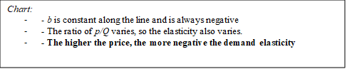
The elasticity is different at every point along a downward-sloping linear demand curve
The elasticities are constant along horizontal and vertical linear demand curves.
When the curve is linear:
To calculate the elasticity of the demand for a linear demand curve, we use this formula:
−b pQ−b pQ
That is, a 1% increase in price causes a larger percentage fall in quantity near the top (left) of the demand curve than near the bottom (right).
Case n°1: when the demand is perfectly inelastic:
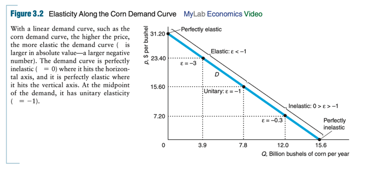 At the beginning of the demand curve (where price is zero and quantity is a constant, a), the demand is perfectly inelastic (e = -b(0/a) = 0.) This means that a 1% increase in price does not change the quantity demanded at all. At a point where the elasticity of demand is zero, the demand curve is perfectly inelastic meaning that if the quantity demanded does not change in response to the price change, it is perfectly inelastic.
(Inelastic means that something doesn't change much when something else changes.)
Case n°2: when the demand is inelastic:
For prices between the midpoint of the linear demand curve and the lower end (where quantity demanded (Q)= a), the demand elasticity falls between 0 and -1. This indicates that a 1% increase in price leads to a decrease in quantity, but the decrease is less than 1%. It's still inelastic, but not perfectly so.
As the price rises, the elasticity gets more and more negative, approaching negative infinity. Where the demand curve hits the price axis, it is perfectly elastic. At the price a/b = $31.20 where Q = 0, a 1% decrease in p causes the quantity demanded to become positive, which is an infinite increase in quantity.
Case n°3: when the demand is horizontal or vertical:
 For a strictly vertical and the strictly horizontal linear demand curves the elasticity is called constant-elasticity demand curves.Ex : if the price goes up or down by, say, 10%, the quantity bought will also change by a fixed 10% proportion. This suggests that consumers are responsive to price changes, and their buying habits adjust in a consistent way regardless of the price level.
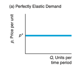
Horizontal Demand Curve: means that people are willing to buy as much as firms sell at any price less than or equal to p* (peut importe la quantiter les consomateur veulent acheter a ce prix la). If the price increases even slightly above p*, the demand falls to zero. Thus, a small increase in price causes an infinite drop in quantity, so the demand curve is perfectly elastic at every quantity.
Why would a demand curve be horizontal?
This type of demand typically happens with products where consumers have many substitutes available, and they can easily switch to other options as soon as the price goes up. As a result, the quantity demanded drops to zero as soon as the price exceeds a certain poverty level.
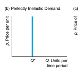
Vertical Demand Curve: is perfectly inelastic everywhere. If the price goes up, the quantity demanded is unchanged (∆Q/∆p = 0), so the elasticity of demand must be zero.
Why would a demand curve be vertical ?
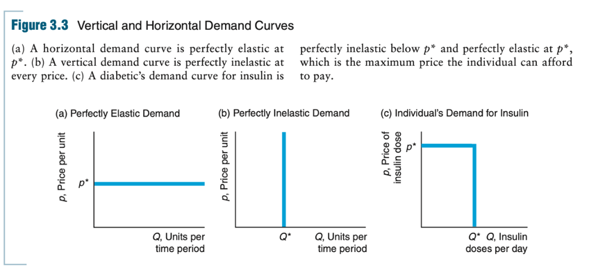 A demand curve is vertical for necessityl goods (goods that people feel they must have and will pay anything to get ex: medicine ).
Demand elasticity and revenue
Elastic demand:P by 1% by more than 1%
`If demand is elastic (a 1% increase in price leads to a more than 1% decrease in QT demanded
Result: Total revenue (PxQ) falls bcuz the % decrease in QT is smaller than the % increase in price
Inelastic demand : P
If demand is inelastic (a 1% increase in price leads to a less than 1% decrease in QT demanded
Result: Total revenue (PxQ) remains the same bcuz the % decrease in QT is smaller than the % increase in price
Unit elastic Demand :P
If demand is inelastic (a 1% increase in price leads to a less than 1% decrease in QT demanded
Result: Total revenue (PxQ) remains the same bcuz the % decrease in QT is equal to the % increase in price
Demand Elasticities over time
The shape of the demand curve depends on the relevant period. A short-run elasticity may differ substantially from a long-run elasticity.
Short-run elasticity: This refers to how responsive consumers are to changes in the price of a product when they don't have much time to adjust.
Long run elastic: refers to how people or businesses respond to changes in price or other factors when they have more time to make adjustments.
Two factors that determine whether short-run demand elasticities are larger or smaller than long-run elasticities are ease (facilitié) of substitution and storage opportunities.
Often “substitute” between products occurs in the long run but not in the short run. Gasoline Example: When gasoline prices dropped significantly, consumers didn't immediately change their driving habits in the short run. However, in the long run, if low prices persisted, people might buy larger cars, take jobs farther from home, or plan more driving vacations.
Storage Opportunities: Some goods can be easily stored, while others can't. For goods that can be stored (like canned foods), consumers might respond more to short-term price changes, buying extra and storing them. Goods that can be easily stored (like frozen orange juice) might see consumers respond more to short-run price changes because they can stock up when prices are low. (short-run demand curves may be more elastic than long-run curves.)
Because demand elasticities differ over time, the effect on revenue of a price increase also differs over time. For example, because the demand curve for gasoline is more inelastic in the short run than in the long run, a given increase in price raises revenue by more in the short run than in the long run.
Revenue Impact: Because demand elasticities differ over time, the effect of a price increase on revenue also varies. In the case of gasoline, a price increase raises revenue more in the short run than in the long run because consumers are less responsive to price changes in the short term.
Other demand elasticities
Income Elasticity of the demand: it measures how much people's demand for a product changes when their income changes
𝜉=percentage cℎange in quantity demandedpercentage cℎange in income
If quantity demanded increases as income rises (the demand curve shifts to the right), the income elasticity of demand is positive.
If the quantity does not change as income rises, the income elasticity is zero.
If the quantity demanded falls as income rises (the demand curve shifts to the left), the income elasticity is negative.
`Cross-Price Elasticity: it’s how the price of one product affects the demand for another product.
x
When the cross-price elasticity is negative, the goods are complements meaning that people will buy less of the good when the price of the other good increases: The demand curve shifts to the left.
Ex: peanut butter and jelly, they're used together. So, when the price of one goes up, people buy less of both.
If the cross-price elasticity is positive, the goods are substitutes. As the price of the other good A increases, people will buy more of good B like Coke and Pepsi, when the price of one goes up, people buy more of the other.
Sensitivity of thr quantity supplied to price
Elasticity of Supply :
The price elasticity of supply (or elasticity of supply) is all about how much more or less of a product a producer is willing to make when the price of that product goes up or down. The elasticity of supply describes the movement along the supply curve as price changes,
= =
where Q is the quantity supplied. (the numerator is Qs for quantity supplied)
Interpretation: If η = 2, a 1% increase in price leads to a 2% increase in the quantity supplied.
If the supply curve is upward-sloping the supply elasticity is positive.
If the supply curve is downward-sloping, the supply elasticity is negative
We use the terms inelastic and elastic to describe the slope of the curves.
If η = 0, we say that the supply curve is perfectly inelastic: The supply does not change as price rises.
If 0< η < 1, the supply curve is inelastic (but not perfectly inelastic): A 1% increase in price causes a less than 1% rise in the quantity supplied.
If η = 1, the supply curve has a unitary elasticity: A 1% increase in price causes a 1% increase in quantity
If η > 1, the supply curve is elastic. If η is infinite, the supply curve is perfectly elastic.
(Unitary elasticity), means that if the price of a product goes up or down by a certain percentage, the quantity producers are willing to supply changes by the exact same percentage in the same direction. For example, if the price increases by 10%, the quantity suppliers are willing to provide also increases by 10%)
The supply function of a linear supply curve is
. = h.
Where g and h are constants. By the same reasoning as before, ∆Q = h∆p, so h = ∆Q/∆p shows the change in the quantity supplied as price changes. Thus, the elasticity of supply for a linear supply function is
Q= g + hp
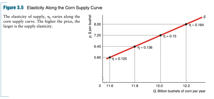
Elasticity along the supply curve
As for the demand, the elasticity of supply varies as well along most linear supply curves. Only constant elasticity of supply curves have the same elasticity at every point along the curve. Vertical and horizontal supply curves are two extreme examples of both constant elasticity of supply curves and linear supply curves.
Horizontal supply curve:
An horizontal supply curve implies that the price elasticity of supply is perfectly elastic. Producers are willing to supply any quantity of a product at a fixed price, and this willingness to supply does not change no matter how much the price changes.
It's an extreme case where producers are very responsive to price changes, and they'll keep supplying the same amount regardless of if the price goes up or down. This is often happens where supply is not constrained by production capacity or other limiting factors, and producers are ready to provide as much as consumers want at a constant price.
Vertical supply curve:
A supply curve that is vertical is perfectly inelastic. No matter how much the price changes, the quantity supplied remains the same. Producers are not responsive to price changes; they are willing to supply a fixed quantity regardless of price fluctuations.
Vertical supply curves typically represent situations where supply is limited by factors other than price, such as production capacity, available resources, or technology constraints. Producers are unable or unwilling to increase their output in response to changes in price, resulting in a perfectly inelastic supply.
Supply elasticities over time
Short-Run Supply Elasticity: This is about how quickly a company can increase its production when people want to buy more. If a company can't easily make more stuff right away, its short-run supply elasticity is low. It's like a restaurant not being able to serve more meals because it's already packed with customers.
Long-Run Supply Elasticity: This is about how much a company can grow and produce more over a longer time. If a company has the time and resources to expand, like building new factories or getting more machines, it can adapt better to changes in demand.
Effects of a sales tax
EX: hospitals might struggle to hire more doctors and nurses right away (short run), but in the long run, they can train more medical professionals or build new facilities to handle more patients. So, the supply of healthcare can be more flexible in the long run because they have time to make changes. It's like planning for a bigger party and having enough time to get more food and drinks.
Governments use two types of sales taxes: ad valorem (VAT) and specific taxes.
Ad valorem (VAT) (21%)/ the sales tax:
Economists call the most common sales tax an ad valorem tax or the sales tax which is the fraction (v) that the government keeps from every dollar the consumer spends on goods.
For example: Japan’s national ad valorem sales tax is 8%. If a Japanese consumer buys a Nintendo Wii for ¥40,000, the government collects v * ¥40,000 = 8% * ¥40,000 = ¥3,200 in taxes, and the seller receives (1 - v) * ¥40,000 = 92% * ¥40,000 = ¥36,800.
(pour connaitre ce que le gouvernement prend je prend le % et je multiplie par la somme a laquelle le produit est vendu.), (Pour savoir ce que le producteur a on fait 1- le % (la taxe) multiplier par le prix du produit)
Specific taxes/unit tax:
Sales tax is a specific or unit tax: The government collects a specified dollar amount, t, per unit of output.
For example, the federal government collects t = 18.4¢ on each gallon of gas sold in the United States.
Effects of a Specific Tax on the Equilibrium:
What effect does a specific sales tax have on equilibrium price and quantity as well as on tax revenue?
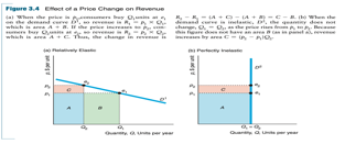
A specific tax causes the price customers pay to go up, the quantity traded to go down, and it generates tax revenue for the government. This means customers and producers are worse off due to the tax, the government benefits by collecting more money. A specific tax causes the equilibrium price customers pay to rise, the equilibrium quantity to fall, and tax revenue to rise.
Example: Imagine the government imposes a tax of $2.40 on each bushel of corn that farmers sell.
Firm's Perspective: Before the tax, farmers were willing to supply 11.6 billion bushels of corn at a price of $5.60 per bushel. This is shown by the supply curve S1.
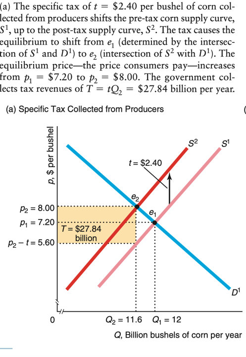
Effect of the Tax: After the tax, if customers pay $5.60, farmers only get to keep $3.20 ($5.60 - $2.40) after paying the tax. So, they are not willing to supply as much corn. To make them willing to supply the same amount, customers must pay $8.00, so that farmers receive $5.60 ($8.00 - $2.40) after the tax. This results in a new supply curve, S2, which is $2.40 higher than S1 at every quantity.
Price and Quantity Changes: The tax leads to changes in the market equilibrium. Before the tax (e1), the equilibrium price is $7.20, and the quantity is 12 billion bushels. After the tax (e2), the new equilibrium price is $8.00, and the quantity is 11.6 billion bushels. So, the tax causes the price customers pay to increase by 80 cents (∆p = p2 - p1 = $8 - $7.20 = 80¢) and the quantity bought and sold to decrease by 0.4 (∆Q=Q2 -Q1 =11.6-12=-0.4). billion bushels.
Tax Revenue: The government collects tax revenue, which is the money it gets from the tax. In this case, it collects $27.84 billion per year. This tax revenue is represented by the shaded rectangle in the diagram, with its height being $2.40 (the tax per bushel) and its width being 11.6 billion bushels (the quantity sold). ($2.40* 11.6 billion bushels per year = $27.84 billion per year)
The Equilibrium Is the Same No Matter Whom the Government Taxes
Are the equilibrium price or quantity dependent on whether the specific tax is collected from suppliers or their customers?
it doesn't matter who pays the tax (suppliers or customers) because the end result, in terms of prices, quantities, and government revenue, stays the same.

Tax from Customers: Imagine customers buy corn at a price of p, and then the government adds a tax of t on top. So, the total price they pay is p + t. If they bought a certain amount (Q) before the tax, they would be ready to keep buying the same amount (Q) only if the price without the tax (p*) drops by the amount of the tax (t). So the after-tax price is still p* - t, which keeps the price for the buyers the same as before.
The Effect on Demand: From the perspective of the companies selling corn, this means the demand (how much buyers want) goes down because the price with the tax is higher. This shifts the demand curve from D1 to D2 in the graph.
Finding the New Balance: The place where the new demand curve (D2) meets the supply curve (S1) is the new balance point, let's call it e3. At this point, the quantity is Q2 = 11.6 billion bushels, and the price farmers get is p2 - t = $5.60.
No Matter Who Pays the Tax: Now, whether you look at this from the customer's perspective (e2) or the seller's perspective (e3), the after-tax balance point is the same. The price customers pay is $8, and the government still collects $27.84 billion in tax money. This means that whether it's the sellers or buyers paying the tax, the end result is pretty much the same.
Firms and Customers Share the Burden of the Tax:
Is it true, as many people claim, that producers pass along to consumers any taxes collected from producers? That is, do consumers pay the entire tax?
Whether the tax burden falls mostly on businesses or consumers depends on how sensitive each side is to price changes.
Tax Incidence: This is about figuring out who really ends up paying for a tax, like when you buy something and there's a tax added. We want to know how much of that extra cost falls on consumers.
The Real Burden: The problem is that the tax on consumers depends on how much the price goes up because of the tax. If prices don't go up much, consumers don't have to pay too much extra because of the tax. But if prices shoot up, consumers are hit harder.
Who Pays More: it's mostly the business or the consumers who pay the tax depends on how quickly they react to price changes.
If businesses are slow to raise prices, they may absorb some of the tax cost.
But if consumers don't change their buying habits much when prices go up (they still buy the same amount), then they end up paying most of the tax.
The Key Players: This all comes down to how sensitive both suppliers (supply) and consumers (demand) are to changes in price.
Tax Effects Depend on Elasticities:
If businesses (supply) have an elastic supply, they can absorb more of the tax, and consumers won't have to pay as much of it because prices won't go up by a lot.
If consumers (demand) have an elastic demand, they can avoid paying too much of the tax by reducing their purchases when prices go up due to the tax.
But, if either supply or demand is inelastic (not very responsive to price changes), then consumers may end up paying most of the tax because prices will go up, and businesses won't change what they produce much.
Ad Valorem and Specific Taxes Have Similar Effects
Do comparable ad valorem and specific taxes have equivalent effects on equilibrium prices and quantities and on tax revenue?
Suppose that the government imposes an ad valorem tax of v, instead of a specific tax, on the price that consumers pay for corn.
We already know that the equilibrium price is $8 with a specific tax of $2.40 per bushel. At that price, an ad valorem tax of v = $2.40/$8 = 30% raises the same amount of tax per unit as a $2.40 specific tax.
It is usually easiest to analyze the effects of an ad valorem tax by shifting the demand curve. Figure 3.7 shows how a specific tax and an ad valorem tax shift the corn demand curve. The specific tax shifts the original, pre-tax demand curve, D, down to Ds, which is parallel to the original curve. The ad valorem tax rotates the demand curve to Da. At any given price p, the gap between D and Da is v.p, which is greater at high prices than at low prices. The gap is $2.40 (=0.3 * $8) per unit when the price is $8, but only $1.20 (=0.3 * $4) when the price is $4.
Imposing an ad valorem tax causes the after-tax equilibrium quantity, 11.6, to fall below the pre-tax quantity, 12, and the post-tax price, p2, to rise above the pre-tax price, p1. The tax collected per unit of output is t = vp2. The incidence of the tax that falls on consumers is the change in price, ∆p = (p2 - p1), divided by the change in the per-unit tax, ∆t = vp2 - 0, collected: ∆p/(vp2). Usually, buyers and sellers share the incidence of an ad valorem tax.
The ad valorem tax of v = 30% has exactly the same impact on the equilibrium corn price and raises the same amount of tax per unit as the $2.40 specific tax, the incidence is the same for both types of taxes.
Subsidies: A subsidy is a negative tax. The government takes money from firms or consumers using a tax, but gives money using a subsidy. Governments often give subsidies to firms to encourage the production of specific goods and services such as certain crops. Since a subsidy is a negative tax, it has the opposite effect on the equilibrium as does a tax.
Chapter 4
Intro
Consumer behavior in microeconomics explores how individual make decisions when faced with limited resources (constraints). It helps predict how consumers respond to changes in prices, income, and other factors.
There are factors that drive people’s preferences.
Trade-offs they make due to budget constraints.
How they seek to maximize their well-being by allocating their resources efficiently
4.1 Preferences
There are 3 basic assumptions to make predictions on consumer preferences:
Completeness: Consumers can rank their preferences for different bundles of goods, ensuring clear and consistent choices.
Transitivity: Consumer preferences are logically consistent, so if they prefer A to B and B to C, they also prefer A to C.
Ex: if you like ice cream more than cake, and cake more than candy, you should also prefer ice cream to candy.
More Is Better (monotonicity): Consumers generally prefer more of a good to less, simplifying the analysis and aligning with the idea that consumers prefer greater quantities of goods when making choices.
Ex : if you enjoy pizza, having more pizza is usually better.
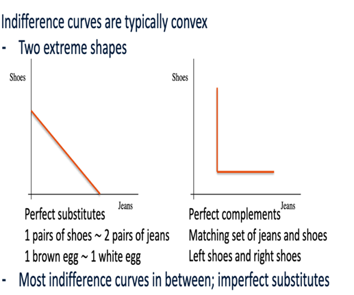 Indifference curves: Are graphical representations of a consumer's preferences. They show all the combinations of two goods that provide the same level of satisfaction or pleasure. Each curve represents a different level of satisfaction. (a line representing equal satisfaction)
They can have different shapes:
Perfect Substitutes: In this case, consumers see two goods as nearly identical, and their indifference curves are straight lines.
EX: if you can't tell the difference between Coca-Cola and Pepsi, you'd be willing to trade one can of Coke for one can of Pepsi.
 Perfect Complements: When goods are consumed together in fixed proportions, the indifference curves have right angles.
EX: Think of pie, where you need one slice of pie for one scoop of ice cream. You wouldn't trade pie for more ice cream or vice versa.
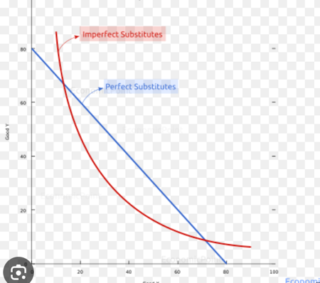
Imperfect Substitutes: a good or service that replaces another but has significant differences. Here, indifference curves are curved and convex (bulging outwards). Consumers are willing to trade between goods, but the rate of trade-off (marginal rate of substitution) decreases as they have more of one good.
EX : Replacing butter with applesauce is an example of an imperfect substitute. It still works as an alternative, but there is a perceivable difference to the consumer.
Marginal Rate of Substitution (MRS): It represents the rate at which a consumer is willing to exchange one good for another while remaining at the same level of satisfaction (on the same indifference curve).
It's calculated as the negative of the slope of an indifference curve. If you're willing to give up some quantity of good A (let's say pizza) to get more of good B (e.g., burritos while staying equally happy, the MRS tells you how many units of A you're willing to give up for one more unit of B `
MRS =
4.2. Utility
Concept that represents the satisfaction or pleasure a consumer gets from consuming a particular bundle of goods.
🡪 DEF :a set of numerical values assigned to various bundles of goods to reflect the consumer's relative ranking of those bundles.
Utility function: summarizes a consumer's preferences by providing a way to calculate the utility of any given bundle.
EX: Lisa's utility function, U(Z, B), tells us how many utils she receives from consuming Z pizzas and B burritos.
Ordinal preference: ranking choices in order of preference without assigning specific numerical values to them. EX: you can say that you prefer ice cream over cake.
Cardinal preference: provides absolute comparisons between ranks by assigning specific numerical values to preferences. Ex: you might say you prefer option A three times as much as option B.
Marginal Utility: the extra utility (satisfaction/happiness) a consumer gains from consuming one additional unit of a good while keeping the consumption of other goods constant.
Ex: Let's say Nolwenn’s eating pizza, and she decides to have one more slice, so she consumes an additional pizza (ΔZ = 1). When she does this, she finds that her total satisfaction or utility (ΔU) increases by 20 "utils,"
In this case, the "Marginal Utility of Pizza (MUZ)" is calculated by dividing the change in total utility (ΔU) by the change in the quantity of pizza consumed (ΔZ):
MUZ = ΔU / ΔZ 🡪 MUZ = 20 utils / 1 pizza = 20 utils per additional pizza.
MU = 🡪
 4.3. Budget Constraint
A budget constraint represents the limit on what a consumer can buy, given their income and the prices of goods.
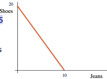
EX: Your budget is €100 jeans cost €10 and shoes €5
10J + 5S = 100
Y= Px(x)+Py(y)
Px/ Py = the prices of goods (x+y)
Y= the total income or budget,
Opportunity set: the collection of all possible bundles of goods that a consumer can buy. It includes bundles within the budget constraint and those on the budget constraint.
(All the possible combinations of goods or services that someone can afford with their available resources, like income or budget.) Tout ce que tu peux acheter avec ton budget.
Ex: Imagine you have $100 to spend on either jeans ($10) or shoes ($5). The opportunity set, in this case, includes all the different combinations of jeans and shoes that you can buy with your $100. You could buy 10 pairs of shoes ($5 x 10 = $50) and 5 pairs of jeans ($10 x 5 = $50) or 5 pairs of shoes ($5 x 5 = $25) and 7 pairs of jeans ($10 x 7 = $70) and more.
Slope of the budget constraint (its equal to the MRT)
The slope of the budget line (budget constraint) depends on the relative prices of the goods.
It reflects the trade-off between the two goods..
This shows how many units of one good Lisa has to give up (or can obtain) to gain (or lose) one unit of the other good.
Effect of changes
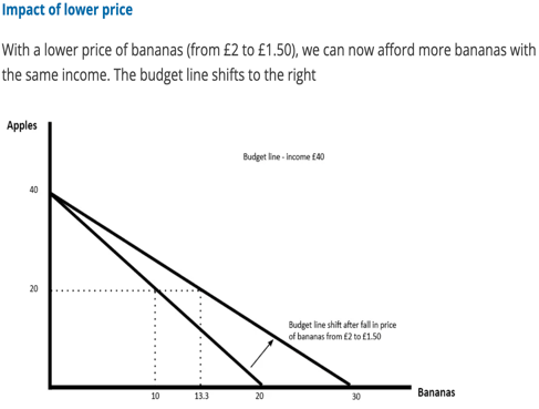
Changes in income, or prices of goods, can affect the position and shape of the budget constraint.
An increase in income shifts the budget constraint outward, while a decrease shifts it inward, assuming prices remain constant.
 Changes in the prices of goods impact the slope of the budget constraint. EX: if the price of pizza increases (while the price of burritos stays the same), the slope of Lisa's budget constraint changes, indicating a different trade-off between pizza and burritos.
Parallel shifts: When income changes, the budget constraint shifts parallel to its original position. Prices do not affect the slope of the constraint; rather, they influence the intercepts on the axes.
4.4. Constrained consumer choice
Consumer optimization: the Fact that consumers aim to maximize their well-being or utility while staying within their budget.
Conditions for optimization: The consumer's optimal bundle occurs when indifference curve is tangent to the budget constraint. This means the consumer is spending the last dollar on each good such that the marginal utility per dollar spent is equal for both goods.
EX:Conditions for Optimization🡪 You make the best choice when you spend all $20 and the happiness from the last $1 spent on ice cream is the same as the happiness from the last $1 spent on chocolate.
Equal Marginal Utility per Dollar🡪 If the last $1 spent on ice cream makes you as happy as the last $1 spent on chocolate, you've found your optimal choice. It's like saying you get the most happiness from your money.
Optimal bundle: For a consumer, it’s a combination of goods and services that provides the highest level of satisfaction (utility) within their budget.
Marginal rate of transformation (MRT): Measures the rate at which a consumer can trade one good for another in the market, given the relative prices of the goods / w/o changing the total production level.
🡪 indicates the amount of one good that must be given up to produce more of the other while maintaining the same overall production level.
MRT=
Convex indifference curve: It means that consumers prefer to have a little bit of both goods rather than just one. So, they like variety and don't want to consume only one good. This assumption helps ensure that consumers choose combinations of goods instead of consuming only one good (corner solution).
4.5 Behavioral economics
Behavioral economics aims to provide a more accurate understanding of economic decision-making, acknowledging that individuals don't always act as perfectly rational beings.
It recognizes that individuals' decisions and preferences are influenced by cognitive biases, emotional attachments, and other psychological factors.
Transitivity: refers to the consistency in decision-making. (In traditional economic theory)
However, behavioral economics has shown that people's preferences can sometimes violate transitivity. This highlights that human decision-making can be influenced by various cognitive biases and emotional factors, leading to inconsistent choices.
Endowment effect: It suggests that people tend to overvalue items they own compared to what they would pay to buy them.
Ex :If you own a coffee mug, you might value it more than you would if you didn't own it. For instance, you might be unwilling to sell your coffee mug for $10, even though you wouldn't pay more than $5 to buy the same mug if you didn't already own it. This is the endowment effect, where ownership increases the perceived value of an item.
This can create a "kink" (refers to a point where the slope of the curve changes abruptly.) in indifference curves, leading to deviations from the traditional rational choice model.
This can occur due to various factors, such as changes in preferences, constraints, or the marginal rate of substitution between goods.
The endowment effect can influence the shape of indifference curves by making individuals less willing to give up items they already own, leading to a change in their preferences and making the curves appear to kink or bend in certain ways.
Salience Effect: refers to the idea that people tend to focus more on information that is prominent, easily noticeable, or emotionally charged.
Chapter 5
EX: You see an advertisement for a fast-food meal, and it highlights a free toy with the meal. The toy is prominently displayed in the ad, making it stand out. As a result, you might be more likely to buy the meal because the toy's offer is so noticeable
Main uses of consumer theory
Determining Demand Curves: Consumer theory helps show the shape of demand curves by manipulating the price of a good while keeping other prices and income constant. This info helps firms set prices and aids governments to predict the impact of policies such as taxes and price controls.
Impact of Income on Demand: Consumer theory illustrates how an increase in income causes the shift of demand curves. Firms use this to predict the increased demand for their products in less-developed countries that experience a rise in income.
Price Change Effects: Consumer theory explains that when the price of a good rises, it affects demand in two ways. Firstly, consumers tend to buy less of the relatively more expensive good, even if compensated for the price increase (substitution effect). Secondly, higher prices reduce consumers' purchasing power, causing them to buy fewer goods overall or alter their consumption patterns.(income effect)
5.1 Deriving the demand curve
Thanks to consumer theory, we know how much less of a good people buy when its price increases. This is derived by examining how consumer choices shift when the price changes while other factors remain constant.
When we change one price but keep everything else the same, we see how much people want to buy. This helps us draw the demand curve. It also connects to how people's preferences affect the curve's shape, called elasticity of demand.
Price-consumption curve: shows how a consumers consumption changes when the price of one of the good changes
🡪 This curve illustrates the various combinations of two different products that a consumer can buy with a fixed income, showing how the changes in prices of these goods influence the quantities that can be bought.
Shapes of PCC
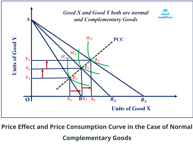
Upward Slope: Both products A and B are consumed more when the price of B decreases. If there is a change in the price of one good (Ex: price of a car in car and petrol) then the demand for it’s complementary good will change in the opposite direction . The PCC in this case is upward sloping showing the inverse relationship between the change in price of one the good and the resulting change in QT demand of it’s complementary good.
Flat Slope : Means that the consumption of both goods A and B remains the same even if the price of B decreases. There's no change in the quantity demanded for either good despite the price change.
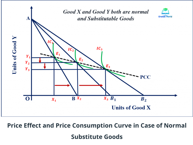
Downward Slope: Consumption of product A decreases while consumption of product B increases when the price of B decreases. These goods are known as substitutable goods , the PCC is downward sloping showing the postive reationship between the change in the price of one commodity and the change in demand for it’s related commodity .
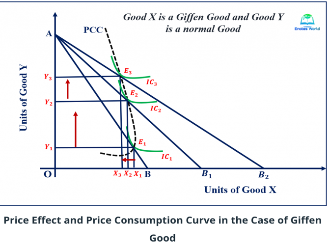
Backward bending : Reflects a situation where the demand for a good decreases with a decrease in its price and increases with an increase in price, defining it as a "Giffen Good." This indicates a positive relationship between price and demand. The resulting Price Consumption Curve (PPC) bends backward, showing that as the price of the Giffen Good decreases, the consumer demands less of it and more of the normal Good Y.
Price consumption curve VS demand curve : the demand curve concentrates on the relationship between the price of a single product and its quantity demanded, while the price consumption curve delves into how price variations of two different goods impact the consumer's purchasing choices, given a constant income.
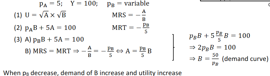
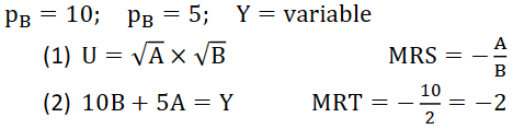
Mathematical aproach
5.2 How Changes in Income Shift Demand Curves
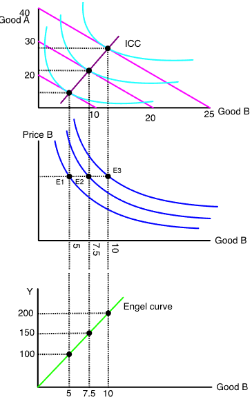
Income elasticities indicate how demand changes when income increases. They help summarize the Engel curve's shape, the income-consumption curve, or demand curve shifts with income changes. Companies use income elasticities to predict how income taxes may affect consumption.
Income elasticities : jnvzjnvznvkjnfrkjfrejknverkjgnerkj
Engel curve : shows the relationship between income + QT demanded of a good
 Asseses how responsive demand is to change income assuming other factors remain constant
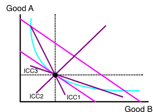
ICC1-> good A normal and good B inferior
ICC2->good A normal and good B normal
ICC3-> good A inferior and good B normal
 How changes in income shift demand curves:
As the income increase, the whole budget shifts to the right. Because pB stays the same, the demand curve shifts right when the income (Y) increase. `
Income-consumption curve: the line that goes through each optimal bundle, it shows how consumption of A/B increase as income increase.
Mathematical approach:
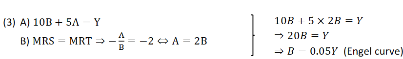
The income-consumption curve showcases how changes in income impact the quantity demanded for different goods while holding their prices constant. The slope of this curve provides insights into the income elasticities of those goods:
Normal Goods : These goods have postive income elasticity (e>0). As income increases (++), the demand for this good also increases (++). The Engel curve for normal goods slopes upward. (positive slope)
Inferior good : This goods have an Negative Income Elasticity (e<0). When income rises (++), the demand for this type of good actually decreases (−−). The Engel curve for inferior goods slopes downward. (negative slope)
Luxury Goods: These are goods with very high income elasticity(e>1). The QTD increases more than proportionally with an increase in income.They are items that people demand more of as their income rises significantly.
Ex : high-end cars, designer clothing, or expensive electronics are often considered luxury goods.
Necessity Goods: These goods have a relatively low income elasticity(0<e<1). The QTD increases when the income increases , but it’s proportionally lower. They are essential items that people need regardless of changes in income.
Ex: Basic food items, utilities, and some healthcare products are often classified as necessity goods.
Normal good turning into inferior good 🡪 A normal good can become an inferior good when people earn more money but start buying less of that good.
Ex: if a person used to eat a lot of fast foods and then, as they earned more, switched to healthier or more expensive food choices like fresh vegetables or restaurant meals causing the demand for fastfood to decline. In this scenario, fast food, which were once a normal part of their diet, become an inferior choice as people's preferences change with their higher income.
5.3 Effects of price change
Substitution Effect: This occurs when the price of a good rises, leading consumers to buy less of that particular good and opt for relatively cheaper alternatives. The idea is to maintain a similar level of satisfaction or utility while adjusting spending due to the price change.
🡪 The change in the quantity demanded of a good due to changes in prices of a good(cause a movement along the utility)
Income Effect: When a price increases, it reduces a consumer's purchasing power. It's similar to a decrease in income because now, with the higher prices, the consumer cannot buy as much with the same amount of money. Even a price increase for one good impacts the consumer's ability to buy the same quantity of all goods they previously bought.
🡪 The change in the quantity demanded of a good due to changes in the income(cause a shift to another indifference curve) (prices are held constant)
EFFECTS WITH A NORMAL GOOD (income/substitution move in the same direction):
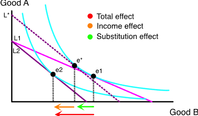 🡪pB increases so the budget constraint goes from L1 to L2, which leads to the optimal bundle to go from e1 to e2. This is the total effect, it can be divided into 2 parts. Assuming the same slope as L2 but with the utility of L1, we get an imaginary optimum at e*with L*. from e1 to e* we have the substitution effect from e* to e2 we have the income effect
The substitution effect is unambiguous hence it will always move into the same direction (hence you will always consume of one more if the other one becomes relatively cheaper)
With the income effect it depends on the type of good which direction it moves (ambiguous direction)
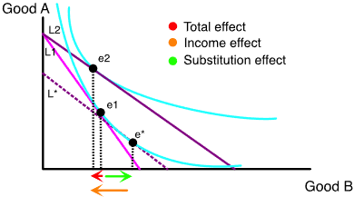 EFFECTS WITH AN INFERIOR GOOD (income/substitution effect move in opposite direction):
Mostly, the income effect is smaller than the substitution effect. The total effect moves in the same direction as the income effect. Giffen good: when p-, d- (basic goods you will replace once your income becomes higher, like rice)🡪violation of the law of demand
Chapter 6
Owners of firms have multiple decisions to make:
Firm structure
Production methods
Expansion strategies 🡪 (short-run adjustments + long-term investments)
The volume of output to produce.
Economic theory helps firms make decision on production process, types of inputs to use and the volume output to produce.
6.1. Ownership and management of the firm
Firms 🡪 Organizations that turn inputs like labor + materials) into goods or services.
Types of firms
Private: owned by people or other nongovernmental entities, whose goal is to make profit
Public: Owned by governments or gov agencies
Non-profit: Organizations that aren’t owned by the government but their goal isn’t to make profit but to pursue social or public objectives. Ex: Greenpeace,
Ownership for profit firms
For-profit firms in the private sector have three main legal structures:
Sole Proprietorship: Owned by a single individual. Ex: Small local shops.
Partnership: Jointly owned and controlled by two or more people. Ex: Law firms.
Corporation: Owned by shareholders who own shares (stock). Shareholders elect a board of directors, who hire managers. Owners have limited liability, protecting personal assets. Ex : Large companies like Apple or Microsoft.
Key feature of corporations is limited liability, (protecting owners' personal assets from the firm's debts) . This concept of limited liability serves as a strong motivator for people to invest in corporations because it minimizes their financial risk. Investors are more willing to buy shares, knowing that their potential losses are confined to the value of their investment.
Limited liability :the personal assets of the owners that can’t be used to pay for a corporation’s debt even if it goes into bankruptcy .
🡪 If a corporation faces financial difficulties or declares bankruptcy, the most shareholders can lose is the amount they invested in buying the company's stock. Their personal assets are shielded from being taken to pay the company's debts.
Management of firms
In small firms, owners often handle management, while larger corporations and partnerships typically have managers or management teams. Decision-making involves owners, managers, and supervisors, each with potentially conflicting objectives.
Ex: a manager may seek benefits that an owner might view as impacting profits negatively.
In corporations, the board of directors oversees managerial decisions, ensuring alignment with the firm's objectives. Shareholders hold the power to replace ineffective managers or influence policies through votes at annual meetings.
What owners want ?
Owners typically aim to maximize profit, represented as the difference between revenue (what the firm earns) and costs (what it pays for inputs). Profit maximization is crucial for staying competitive. Efficient production, achieving technological efficiency, is necessary for profit maximization. It means producing the current output level with the least amount of inputs based on existing knowledge.
While efficient production is necessary, it alone doesn't ensure profit maximization. Managers, often guided by economic decisions, determine how to produce at the lowest cost or with the highest profit(. This involves strategic choices in technology and input combinations.
6.2. Production
Firms use technology or production process to transform inputs (factors of productions) into outputs.
Here are the different types of inputs:
Capital services (K): Long-lived inputs like land, buildings, and equipment.
Labor services (L): Hours of work from managers, skilled, and less-skilled workers.
Materials (M): Natural resources, raw goods, and processed products consumed or incorporated in the final product.
Production function
Firms have many ways of transforming inputs into output. The production function shows the relationship between the number of inputs used and the maximum output that can be achieved
q=f(L,K)
🡪 The production function showcases the maximum output possible with given levels of labor and capital, focusing on efficient production processes. A profit-maximizing firm avoids inefficient processes and aims to use resources optimally.
Ex: Consider a smartphone manufacturing company with multiple production methods. In smaller setups, skilled workers assemble phones manually, while larger firms may introduce automated assembly lines. In advanced facilities, robots and advanced machinery, maintained by skilled technicians, handle intricate assembly processes.
The production function for such a firm, involving labor (L) and capital (K), might be expressed as q=f(L,K)),
q= nbr of smartphones produced
L= labor services 🡪 skilled + unskilled workers
K= capital 🡪 machinery + technology
Varying inputs over time
It’s easier for a firm to adjust its inputs in the long run than in the short run, because in the short run, a firm faces limits in adjusting its inputs, with at least one factor being practically unchangeable. This fixed factor is a fixed input, while those that can be easily adjusted are variable inputs. Conversely, the long run allows a firm to vary all factors of production.
Ex : consider a painting company with a fixed number of trucks and compressors for a day's work. In the short run, it might deploy its existing resources more efficiently. However, in the long run, the company can adjust all inputs, hiring more workers, acquiring additional trucks and equipment, and improving project tracking.
In different industries, the time it takes to change inputs varies. Janitorial firms, focusing on labor-intensive services, can adjust quickly in the long run. However, industries like automobile manufacturing might take years to build new plants or create specialized machinery.
In the short term, materials and often labor are flexible inputs for many firms. But labor flexibility depends on available skills. Capital can also be flexible (like renting trucks) or fixed (like building structures), and the time needed to adjust varies accordingly. This shows that firms can adapt more in the long run compared to the short run.
short run: a period so brief that at least one factor of pro- duction cannot be varied practically.
fixed input: a factor of production that the firm cannot practically vary in the short run.
variable input: a factor of production that the firm can easily vary during the relevant period
long run: a lengthy enough period that all factors of production can be varied.
6.3. Short run production
In the short run, a company has fixed inputs, like capital or factory space, that can’t be altered immediately due to contractual obligations, technological constraints, or time needed for changes.
Companies may use the short run to make immediate production adjustments by varying only the variable inputs like labor, raw materials, or energy consumption.
Ex : hiring or firing workers, using overtime, or adjusting the quantity of raw materials without changing the overall capacity of the factory.
.
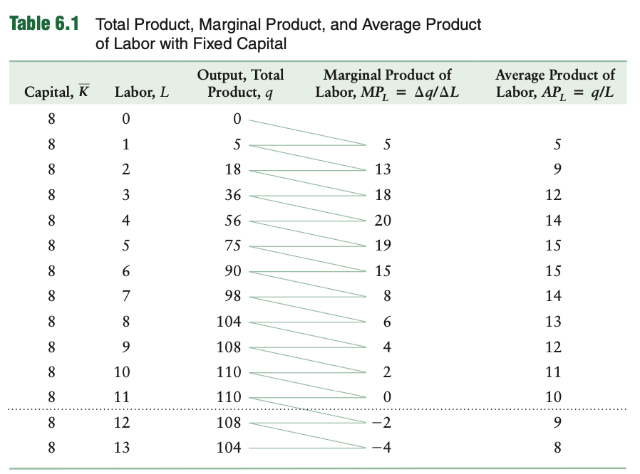
Scenario: a firm assembling computers with fixed capital (eight fully equipped workbenches) and variable labor. The short-run production function is given by q=f(L,K) where q is the output, LL is the amount of labor, and K is the fixed capital.
🡪 as shown in Table 6.1, with zero workers, no computers are assembled. Adding workers initially increases output, reaching a maximum of 110 computers per day with 10 or 11 workers. However, employing more than 11 workers becomes inefficient, decreasing production.
Marginal Product of Labor
a concept used to understand how an additional worker affects total output. Represents the extra output produced from adding/ hiring one more unit of labor (worker)
MPL=∆q/∆L
EX: in Table 6.1, when the number of workers increases from 1 to 2 (∆L=1∆L=1), the output rises by ∆q=18−5=13. Therefore, the marginal product of labor is MPL=13/1=13.
In the short run, where capital is fixed, the focus is on how changes in labor impact output. Understanding MPL helps managers make decisions about hiring additional workers based on their contribution to overall production
Average product of labor
The average product of labor (APL) is another crucial measure for firms, representing the ratio of output (q) to the number of workers (L) used in production.
Represents the average output produced per unit of labor input.
🡪 provides insight into the productivity of labor, indicating how much output, on average, each unit of labor contributes to the production process.
APL=
EX: The output (q) is given by 2L+1002L+100.
To determine APL:
Calculate APL: APL=qL=2(L+ΔL)+100L+ΔLAPL=Lq=L+ΔL2(L+ΔL)+100 Simplifying this expression yields APL=2APL=2.
Determine Marginal Product of Labor (MPL): To find MPL, considering an increase in workers by ΔLΔL, the change in output is Δq=2ΔLΔq=2ΔL. Thus, MPL=ΔqΔL=2MPL=ΔLΔq=
Graphing the product curves
 In Figure 6.1, the production relationships with variable labor are illustrated. The total product curve (panel a) shows the amount of output that can be produced by a given amount of labor, reaching its peak at 110 computers with 11 workers. The dashed line indicates inefficient production with more than 11 workers.
Panel b of Figure 6.1 demonstrates the variation of the average product of labor (APL) and marginal product of labor (MPL) with the number of workers. The APL initially rises, indicating that output increases more than in proportion to labor due to factors like specialization. However, beyond a certain point, the APL falls as output increases less than proportionally to labor.
Geometric Relationship of Curves:
Average Product and Marginal Product:
The Average Product of Labor (APL) curve intersects the Marginal Product of Labor (MPL) curve at a point (denoted as 'a').
At this point of intersection, the average product (APL) curve peaks, signifying the highest average output per worker, and the marginal product (MPL) equals the average product.
Beyond this point, the average product starts declining because the marginal product falls below the average product.
If AP=MP then AP at max. :
If MP>AP then AP increasing : When MPL is higher than APL, adding more workers increases average productivity.: When MPL equals APL, adding more workers doesn't change average productivity.
If MP < AP then AP decreasing : When MPL is less than APL, adding more workers decreases average productivity.
Average Product and Total Product:
The slope of the line from the origin to any point on the Total Product of Labor (TPL) curve for a specific quantity of workers represents the Average Product of Labor (APL) for that particular number of workers.
EX ; if you draw a line from the origin to a point on the TPL curve that corresponds to a certain number of workers, the slope of this line gives you the APL for that specific quantity of workers.
Marginal Product and Total Product:.
The slope of the tangent line to the Total Product of Labor (TPL) curve at a specific point represents the Marginal Product of Labor (MPL) at that particular level of output
If you draw a tangent line to the TPL curve at a specific quantity of workers, the slope of this tangent line gives you the MPL at that level of labor input.
when MP > 0 then TP is increasing. : When Marginal Product (MP) is positive (+), it means that adding more workers leads to an increase in Total Product (TP). Each additional worker contributes positively to the total output.
When MP < 0 then TP is decreasing. : When MP becomes negative (-), it implies that further additions of workers result in a decrease in Total Product. This happens when additional workers cause inefficiencies or hinder the production process.
When MP is at max then TP is at inflection point : At the maximum point of MP, Total Product (TP) reaches an inflection point, indicating the highest rate of change in TP. This inflection point represents the peak of productivity concerning the number of workers hired.
When MP = 0 then TP is at a max : When MP reaches zero (0), Total Product (TP) is at its maximum. This occurs because MP turning from positive to zero signifies that adding more workers no longer increases output, indicating the peak of production efficiency.
Law of diminishing marginal return
The Law of Diminishing Marginal Returns states that as a firm increases a particular input while holding other inputs and technology constant, the corresponding increases in output will become smaller eventually. So, if only one input is increased, the marginal product of that input will diminish over time.
EX: In Table 6.1, as the firm goes from 1 to 2 workers, the marginal product of labor increases (from 13 to 18), but beyond a certain point (4 workers), it starts to fall. The law of diminishing marginal returns suggests that each additional worker contributes less and less to the total output.
Diminishing Marginal Returns vs. Diminishing Returns:
Diminishing marginal returns is when you add more of something (like labor or resources) while keeping other factors constant, each extra bit you add doesn't boost production as much as the previous ones did. However, this doesn't automatically mean that the total amount produced will decrease. It might still increase, but at a decreasing rate.( while there might still be an increase, it's happening at a slower pace compared to before.)
It's a concern because adding more of a particular input might not increase production by as much as before. But in real life, advancements in technology and using different inputs together that can help lessen this effect.
EX: in farming, using better techniques or combining different resources can help maintain or increase overall production despite facing diminishing returns from each additional unit of input.
6.4. Long run production
In the long run, both labor and capital are variable inputs, allowing a firm to produce a given level of output through different combinations of these inputs. This flexibility allows for substitution between inputs, similar to how consumers can substitute between goods to maintain a certain level of utility.
In Table 6.2, various combinations of labor (L) and capital (K) are presented, each resulting in the production of 24 units of output per day. The table illustrates how the firm can achieve the same output level with different mixes of labor and capital. EX:
(a) 1 worker and 6 units of capital,
(b) 2 workers and 3 units of capital,
(c) 3 workers and 2 units of capital,
(d) 6 workers and 1 unit of capital.
This ability to adjust inputs allows firms to choose production methods that suit their efficiency and cost considerations in the long run.
Isoquants
DEF: represents the different combinations of labor and capital that allow a firm to produce a specific level of output.
🡪shows combinations of K+L and the technological tradeoff between the 2
(How much capital would be required to replace a unit of labor a a certain production point to generate the same output ?).
Isoquants share several properties with indifference curves, which are used in consumer theory.
Isoquant vs indifference curves 🡪 The difference is that isoquants maintain a constant level of output, while indifference curves maintain a constant level of satisfaction or utility.
Properties of isoquants:
Output Level: Isoquants farther from the origin signify higher levels of output. This is because the firm utilizes more inputs efficiently to achieve increased production.
Non-crossing: Isoquants do not intersect or cross. This property ensures efficiency because if two isoquants were to intersect, it would imply that the same level of output could be produced with the same combination of labor and capital, violating the principle of efficiency.
Downward Sloping: Isoquants slope downward. This characteristic is essential because it reflects the trade-off between labor and capital. As more of one input is used, less of the other is required to maintain the same output level.
Shape and Substitutability: The curvature of isoquants demonstrates the firm's ability to substitute one input for another.
Perfect substitutes : result in straight-line isoquants,
fixed-proportions production functions (no substitutes) : lead to right-angle isoquants.
Most isoquants are convex, sloping downward and curving away from the origin, indicating imperfect substitution between inputs.
In all, isoquants provide a visual representation of a firm's production capabilities and the various combinations of labor and capital that lead to constant output levels.
MRTS(slope of isoquant) : Measures how easily a firm can exchange ne inout for another while keeping output constant
MRTS=
Illustration: In Figure 6.4, the isoquant for a service firm producing 10 units of output is examined. The points a, b, c, d, and e represent different combinations of labor (L) and capital (K). The slope of the isoquant at each point corresponds to the MRTS.
Substitution Example: Moving from point a to b, the firm can produce the same output using six fewer units of capital (∆K = -6) if it hires one more worker (∆L = 1). Therefore, the MRTS at this point is -6.
As the firm increases labor along the isoquant (EX: moving from b to c or c to d), the MRTS declines.
🡪Diminishing MRTS : implies that each additional worker contributes less to the reduction in the use of capital, highlighting the challenge of replacing remaining capital with labor.
Special Case: Isoquants with perfect substitutes do not exhibit diminishing MRTS since the inputs remain perfect substitutes, and neither becomes more valuable in the production process.
6.5. Returns to scale
Returns to scale refers to how changes in inputs like labor and capital affect the output in a production process that employs the same technology. It's a way to measure how efficiently a firm can convert inputs into outputs.
Increasing Returns to Scale:
If a firm doubles its inputs (EX:labor, capital) and output more than doubles.
This implies that as the firm expands its scale, it becomes more efficient, possibly benefiting from factors like specialization and resource pooling.
f(2L,2K)= 2f(L,K) = 2q
Ex: a software development company that enhances its workforce by 20% and, as a result, experiences a 30% increase in developed software products. This scenario reflects increasing returns to scale, possibly due to improved collaboration among team members or specialized skills that enhance productivity as the team grows.
Constant Returns to Scale:
If a firm doubles its inputs and output exactly doubles, it indicates constant returns to scale.
This suggests that the firm maintains the same level of efficiency as it scales up, achieving a proportional increase in output.
Ex : Imagine a pizza shop that doubles both its oven capacity and the number of chefs while keeping all other factors constant. If this doubling of inputs results in exactly double the number of pizzas produced without any change in efficiency, it demonstrates constant returns to scale.
Decreasing Returns to Scale:
occur when doubling inputs results in less than a doubling of output.
This implies that as the firm expands, efficiency may decline due to issues like coordination challenges or diminishing returns to inputs.
Ex : a factory that manufactures furniture. If the factory doubles its production capacity by expanding its machinery and labor force but sees only a 50% increase in the furniture output, it signifies decreasing returns to scale.
Varying returns to scale
The variation in returns to scale showcases the complexity of production dynamics as firms change in size. Small firms benefit from growth and specialization, but as they expand, challenges related to management and coordination might arise, leading to diminishing returns.
6.6. Productivity + technical change
Differences in technology and managerial practices contribute to variations in firms' output from the same inputs. Technological advancements and managerial innovations enable firms to increase productivity, producing more with the same resources. This phenomenon is known as technical change or technological progress. Firms embracing these changes often outperform others by optimizing their production processes.
Relative productivity
Efficiency is crucial for maximizing profit, but firms within a market might still differ in productivity. Factors like management strategies, access to innovations, and external influences can impact relative productivity. Market competition plays a significant role – in competitive markets, less productive firms exit, leaving equally productive ones. In less competitive markets, firms with varying productivity levels may coexist. Factors such as work rules, discrimination, regulations, or institutional restrictions can influence relative productivity among firms.
Innovations
the pursuit of efficiency, firms strive to incorporate the latest technological and managerial advancements in their production processes. Technical progress, arising from innovations, enables firms to produce more output with the same inputs. Whether through new inventions, technical innovations like robotics, or improved management practices, technical progress plays a vital role.
Ex: a firm may produce 10% more output this year with the same inputs due to a new invention.
There are different types of technological progress :
Neutral Technical Change:a technological improvement or advancement that increases productivity without favoring any particular type of input over others. It equally affects all factors of production, like labor and capital, leading to an overall increase in efficiency without changing the ratio of inputs used in production.
Non-neutral Technical Change: When innovation affects the productivity of one input but not the other
Ex: if a company has a new machine that boost the productivity of capital but reducs labor because of the implementation of the machine they need less workers (labor saving technical change)
There are 2 steps that a firm takes in order to choose how to produce outputs efficiently:
IdentifyingTECHNOLOGICALLY EFFICIENT Production Processes: The firm aims to find the most effective and efficient ways to produce a specific output level.
selecting the most ECONOMICALLY EFFICIENT production process among the technologically efficient options: jAfter finding effective ways to produce what they want, the firm picks the most cost-efficient method. They use info from how inputs create output (production function) and input costs to choose the way that minimizes expenses while keeping output at the desired level. It's about finding the cheapest way to make things without compromising on the quantity they want to produce.
economically efficient :minimizing the cost of producing a specified amount of output
Chapter 7
7.1. The nature of costs
Cost analysis in economics involves measuring a company's expenses related to production. Economists and business professionals differ in how they evaluate costs. Economists consider all relevant costs, while managers often focus on financial statements tied to tax laws and shareholder interests.
To create products, a company spends on inputs like labor, capital, energy, and materials. The cost of each input is found by multiplying its price by the quantity used. For instance, if labor costs $20 per hour and the firm uses workers for 100 hours, the labor cost would be $20 * 100 = $2,000 per day. These are explicit costs, representing direct payments for inputs.
Explicit costs : These are the straightforward, tangible costs, like the money spent on purchasing machinery. Ex: rent , material, wages
Implicit costs : are not actual cash payments but represent the value of opportunities a business misses when it uses its resources in a certain way. They are about what the company gives up by choosing one option over another. (They're the opportunity costs—the benefits or profits a company forgoes by choosing one alternative over another.)
Ex if a business owner decides to use their own building for their company instead of renting it out to another business, the implicit cost is the potential rental income they've given up.
Opportunity cost
Opportunity cost : the value of the best alternative use of a resource. It encapsulates both explicit costs (direct, out-of-pocket payments for inputs) and implicit costs (opportunity value of forgone alternatives).(I t's the cost of choosing one option over another)
Ex; If you decide to buy a pizza instead of a burger, the opportunity cost is the taste of the burger that you gave up by choosing the pizza.
EX: imagine Maoyong, who owns a firm, pays himself a salary of $1,000 monthly but could earn $11,000 elsewhere. The opportunity cost of his time isn't the $1,000 he pays himself but rather the $11,000 he could earn elsewhere, highlighting the concept of opportunity cost.
Finding opportunity cost means figuring out what you miss out on by choosing one thing over another. It's about understanding the benefits you give up from the options you didn't choose.
Scenario-🡪 Meredith's firm sends her to a conference, including a free class on pricing derivative securities. However, she could attend a talk by Warren Buffett at the same time. Meredith values Buffett's talk at $100 but the ticket costs $40. If she chooses the derivatives class, her opportunity cost is $60 ($100 - $40), representing the benefit she gives up by not attending Buffett's talk.
Opportunity cost of capital
Opportunity cost of capital refers to the value of the best alternative use of durable assets like equipment or land, typically used over a long period. Determining this cost involves considering allocation of purchase cost and accounting for changes in asset value over time.
Ex: When a company chooses to rent capital assets (such as machinery, vehicles like trucks, or equipment), the monthly rental payment it makes essentially represents the cost the company incurs to use that particular asset for a month. This rental payment reflects the opportunity cost, as it signifies the value of using that asset for that period.
Renting capital assets simplifies the financial aspect for the company. Instead of dealing with the complexities of allocating or spreading out the purchase cost of an asset over its entire useful life, which is the case when buying it outright, the rental cost is a clear and immediate expense. This simplicity in accounting helps in managing and understanding the ongoing monthly expenses more easily.
Sunk Cost: It's money spent in the past that cannot be recovered. Sunk costs have already occurred.
Ex : Buying a gym membership for a year and then deciding not to go anymore. The money spent on the membership is a sunk cost because it's already paid and cannot be recovered, regardless of using the gym or not.
7.2. short-run costs
In the short run, a firm faces costs that increase as it produces more. It's more expensive to increase output in the short run because certain inputs, like capital, cannot be adjusted. This contrasts with the long run, where all inputs are flexible.
Short run cost measures
To produce a given level of output a firm incurs costs for fixed and variable inputs (in the
Shortrun :
a firm faces fixed costs that stay the same regardless of output and variable costs that change with the quantity of output produced.
Ex: expenses for resources that can't be adjusted in the short run, like land or equipment.
VC= w x L
Variable costs:fluctuate with the level of output, involving items such as labor and materials.
The total cost (TC) to produce a specific quantity of output is the sum of fixed cost (F) and variable cost (VC).
EX: if a firm has a fixed cost of $48 and a variable cost that rises from $25 for one unit to $46 for two units, the total cost for producing two units would be $94 ($48 + $46).
TC= F+VC
To decide how much to produce, a firm uses several measures of how its costs varies with the level of output.:
or w x L/Q
Marginal cost (MC): is the change in total cost when producing one more unit of output. It helps firms decide if it's profitable to adjust their output.
FC/Q or w x L/Q
Average fixed cost (AFC) : is the fixed cost divided by the number of units produced, decreasing as output increases.
VC/Q
Average variable cost (AVC): is the variable cost divided by the quantity of output produced, fluctuating with output changes.
Average cost (AC) or average total cost : is the sum of AFC and AVC, showing the overall cost per unit of output. These cost measures assist firms in determining their profitability concerning the price they receive for their products.
TC/Q
Short run cost curves
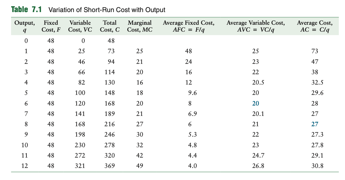
The short-run cost curves show different types of costs a firm faces at various output levels. In Figure 7.1, Panel a shows fixed cost as a horizontal line at a constant value ($48), while the variable cost curve starts from zero and rises with output. The total cost curve, representing the sum of fixed and variable costs, runs parallel to the variable cost curve.
Panle A
Fixed Cost Curve 🡪 A straight line representing costs that do not change with changes in output. It remains constant regardless of the production level.
Variable Cost Curve 🡪 Starts at zero when production is at zero and increases with output because these costs vary with the number of units produced.
Total Cost Curve 🡪 is a parallel line to the VC-curve, which is “amount of the FC” higher than the VC.
Panel B
Average Fixed Cost curve 🡪 Decreases/falls as output rises because the fixed costs are spread over more units as production increases.
Average Cost curve 🡪 Sum of the Average Fixed Cost curve and the Average Variable Cost Curve
Falls when MC < AC and rises when MC > AC
Marginal Cost Curve 🡪 the slope of tangent TC is equal to the slope of the tangent VC
Average Variable Cost curve 🡪 slope of line through origin and VC
It falls when the MC < AVC and it rises when MC > AVC
MC intersects AVC at its min
The Relationship Between Marginal Cost and Average Cost:
When MC is below ATC or AVC, the average cost decreases.
When MC is above ATC or AVC, the average cost increases.
At the minimum point of the average cost curve, MC equals ATC.
The production function defines a firm's cost curves. It shows the relationship between inputs required to produce a specific output level.
In the short run, a company deals with costs that can be changed based on production levels. These costs are termed as variable costs. A key variable cost for many companies is labor expense, which changes based on the number of hours worked by employees and their wage rate.
Variable Cost (VC) = Wage per hour (w) * Number of hours of labor (L)
Ex: if a firm pays its workers $15 per hour and employs 100 hours of labor, the variable cost would be $15 * 100 = $1,500.
Variable Cost Curve: It shows how costs go up when a company hires more workers. As more workers are hired, the cost for each additional worker might not produce as much extra output, leading to higher costs per unit.
Marginal Cost (MC) Curve: This displays how the cost changes when making one more product. At first, adding more workers might reduce costs because they're more productive. But beyond a point, adding more workers leads to less extra output for each new worker, causing costs to rise.
Average Variable Cost (AVC) Curve: It shows the cost per item produced. When each worker produces more, the cost per item decreases, and when each worker produces less, the cost per item increases.
Average Total Cost (AC) Curve: This combines fixed and variable costs. It forms a U-shape because at low levels of production, fixed costs spread over fewer items, and at high levels, diminishing returns cause variable costs to rise per item
The relationship between these curves is such that:
When the Marginal Cost is below the Average Cost, the Average Cost tends to decrease.
When the Marginal Cost is above the Average Cost, the Average Cost tends to increase.
If Marginal Cost equals Average Cost, the Average Cost curve is at its minimum point.
Taxes
Impact of Tax on Costs:
If a tax is imposed per unit of output (e.g., $10 per unit), it increases both average variable cost (AVC) and average cost (AC) by that tax amount ($10).
Marginal cost (MC) and average cost curves shift upward by the tax amount. However, the points where these curves reach their lowest (minimum) values don't change despite the tax increase.
Franchise Taxes' Effect:
Franchise taxes, which are fixed lump-sum payments unrelated to output, only impact fixed costs.
These fixed taxes don't influence how costs change with each extra unit produced (marginal cost curve) but affect the fixed cost part of the average cost curve.
As a result, after-tax average cost curve reaches its minimum at a higher production level compared to the before-tax curve due to the additional fixed tax payment.
7.3 Long-Run Costs
All Costs are Avoidable in the Long-Run
🡪fixed costs in the long-run are avoidable (rather than sunk, as in the short run)
Fixed Costs in the Short Run:
In the short run, fixed costs are often considered sunk costs.
Example: Rent payments for a restaurant space, which remain unchanged regardless of whether the restaurant operates or not. These costs are unavoidable in the short run.
Fixed Costs in the Long Run:
However, in the long run, fixed costs are avoidable.
Example: The same rent for the restaurant space can be avoided in the long run by shutting down the restaurant. Unlike the short run, where the rent is paid irrespective of operations, in the long run, the firm has the flexibility to avoid such fixed costs by ceasing operations.
The difference between the short run and the long run regarding fixed costs is that in the long run, a firm has more flexibility and can adjust its costs, including avoiding certain fixed costs by making different decisions such as shutting down operations.
Long Run Total Cost Equals Long-Run Variable Cost:
In the long run, the total cost of production is equivalent to the long-run variable cost.
This denotes that all costs incurred in the long run, when the firm can adjust all inputs including capital, are considered variable costs. There are no fixed costs in the long run.
Lower Long-Run Cost When Using "Wrong" Capital in Short Run:
Sometimes, when a business can't adjust certain things (like equipment or machinery) in the short term, it might end up spending more money than necessary.
But when it has the chance to adjust everything in the long term, it might spend less because it can make better choices about how it uses its resources.
Minimising Costs
• A firm can produce a given level of output using many different technologically efficient
combinations of inputs, as summarized by an isoquant
• From the technologically efficient combinations of inputs, a firm wants to choose the bundle withthe lowest cost of production →the economically efficient combination of inputs.
A company can make the same amount of stuff using various combinations of tools, workers, and resources.
Out of all these combinations that work efficiently, the company aims to pick the one that costs the least to produce - that's the most economical way to make their product. This chosen combination is called the economically efficient mix of inputs.
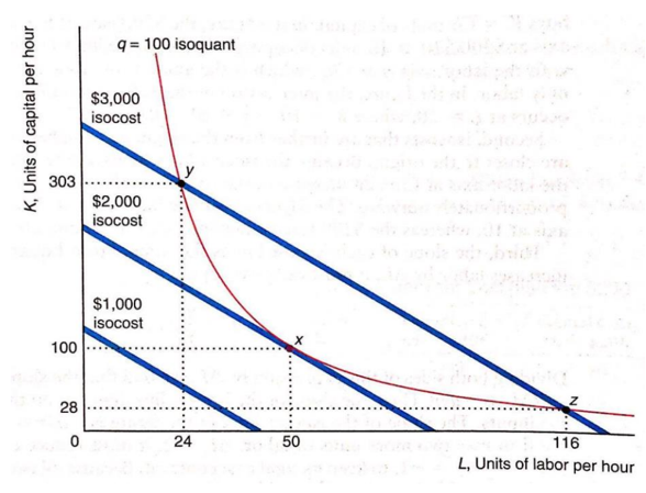 Isocost Line
All the combinations of inputs that require the same (iso) total expenditure (cost)
The cost of producing a given level of output depends onthe price of labour and capital
C = wL + rK.
3 properties:
Where the isocost line hits the axes depends on the firm’s cost
and on the input prices.
Isocosts farther from the origin have higher costs.
Slope of each isocost is the same; if a firm increases labour,decreases in capital
∆K = -w/r ∆L or ∆K/∆L = -w/r
→slope depends on input prices
both isocosts and budget lines are straight lines whose slopes depend on relative prices
difference: consumer has a single budget line determined by income, while a firm faces many
isocost lines each of which corresponds to a different level of expenditures it might make.
Combining Cost and Production Information
The firm can use any of three equivalent approaches to minimise its cost:
Lowest-Isocost Rule:
Pick the bundle of inputs where the lowest isocost line touches the isoquant
firm minimises its cost by using the combination of inputs on the isoquant that is on the lowest isocost line that touches the isoquant
If an isocost line touches the isoquant twice, there must be another lower isocost line that also touches the isoquant
Tangency Rule
Pick the bundle of inputs where the isoquant is tangent to the isocost line
Firm chooses the input bundle where the relevant isoquant is tangent to an isocost line to
produce a given level of output at the lowest cost
To minimise its cost of producing a given level of output, a firm chooses its input so that the
MRTS equals the negative of the relative input prices: MRTS = - w/r.
Last-Dollar Rule
Pick the bundle of inputs where the last dollar spent on one input gives as much extra
output as the last dollar spent on any other product. The tangency rule can be interpreted
in another way: MRTS = - w/r = - MPL/MPK MPL/w = MPK/r.
If the isoquant is not smooth, the lowest-cost method cannot be determined by using the tangency rule or the last-dollar rule
The lowest-isocost rule always works, even when isoquants are not smooth
Factor Price Changes
The change in a price does not affect technological efficiency, so it does not affect the isoquant, only the isocost line is different
The Long-Run Expansion Path and the Long-Run Cost
Function
Expansion path: line through the tangency points,the cost-minimising combinations of labour and capital for each output level.
long-run cost function shows relation between the cost (isoquant) and the total output (isocost line).
The Shape of Long-Run Cost Curves
shapes of the average cost and marginal cost curves depend on the shape of the long-run cost curve
The long-run average cost curve falls when the long-run marginal cost curve is below it and rises when the long-run marginal cost curve is above it.
the marginal cost crosses the average cost curve at the lowest point on the average cost curve
Why does the average cost curve first fall and then,rise? →key reason is that the average fixed cost
7.4 Lower Costs in the Long Run
A firm’s long-run decisions determine its short-run cost. Short-run cost is at least as high as long run cost and is higher if the “wrong” level of capital is used in the short-run.
Long-Run Average Cost as the Envelope of Short-Run Average Cost Curves
long-run average cost is always equal to or below the short-run average cost – if there are many possible SRAC, the LRAC will be smooth and U-shaped
the LRAC includes one point from each possible short-run average cost curve. This point, however,is not necessarily the minimum point from a short-run curve
Short-Run and Long-Run Expansion Paths
long-run cost is lower than the short-run cost because a firm hasmore flexibility in the long run
short-run: firm can only change input of one variable, therefore, the expansion path of short-run output is horizontal – to double its output, it must increase its labour
relatively more and cost doubles relatively more
long-run: doubling inputs, doubles output, the long-run expansion
path is upward sloping
The Learning Curve
• Learning by Doing: the productive skills and knowledge that workers and managers gain from
experience
• A firm’s average cost may fall over time due to learning by doing
• Learning is a function of cumulative output: the total number of units of output produced since the
product was introduced
• Learning Curve:
• relationship between average costs and cumulative output
• If a firm is operating in the economies of scales section of its average cost curve, expanding output
lowers its cost for two reasons
• Its average cost falls today because of economies of scale, and for any given level of output, its
average cost is lower in the next period due to learning by doing.
Task 7 Q5 How is the long run total cost curve related to production function?
The production function shows how much can be produced with different amounts of inputs (like labor and machines).
The long-run total cost curve displays the lowest possible cost for making those amounts of products with varying input combinations.
So, the long-run total cost curve is related to the production function because it shows the costs linked to the different levels of output determined by the production function.
Top of Form
Bottom of Form
Q7 how Short run + lo,g run related ?
The relationship lies in how short-run costs influence long-run costs. For instance, decisions made in the short run, like hiring more workers, can affect long-run costs by influencing factors such as gaining experience or setting up training programs. Long-run costs can be seen as an accumulation of short-run decisions and their effects on overall production efficiency and costs over time.
The connection between them is that short-run costs are part of long-run costs. Long-run costs consider both fixed and flexible aspects of production, while short-run costs only focus on the fixed parts. When decisions are made in the short run (like hiring more workers), they can affect the overall long-run costs by influencing how production is managed over time.
Learning Goals:
How does an economist measure costs, and what’s wrong about the innkeeper’s quote?
Economists measure costs in the short run by considering fixed costs (which don't change with output) and variable costs (which change with the quantity of output produced). The innkeeper's quote might be inaccurate if it only considers the immediate expenses without including the fixed costs, leading to an incomplete understanding of the total cost.
What are the two components of short-run total costs?
Fic-xed costs : don’t vary w/ thee output always the same ex: capital)
Variable costs: they vary with output
3. How are short-run total costs related to the variable production factor?
4. What are average and marginal costs?
5. How are the total, variable and marginal cost curves related to each other?
6. How are the cost curves related to the short-run production function?
7. Determine all the relevant short-run cost curves for the Steinway example in the task.
8. Use the results at 7 to check the relations discussed at 5 and 6.
1. Economists measure costs using various methods such as analyzing explicit costs (direct expenses like rent, wages) and implicit costs (opportunity costs like owner's time or capital), calculating total costs, average costs, and marginal costs associated with producing goods or services. The innkeeper's quote overlooks implicit costs like the opportunity cost of owning the place and not paying rent, and the value of their own labor.
2. The two components of short-run total costs are fixed costs (FC) and variable costs (VC). Fixed costs remain constant regardless of the level of output in the short run, while variable costs change with the level of production.
3. Short-run total costs are related to the variable production factor because variable costs directly depend on the level of the variable input, such as labor or materials, required to produce output. As production increases, variable costs tend to increase due to the need for more variable inputs.
4. Average costs represent the cost per unit of output produced, calculated by dividing total costs by the quantity of output. Marginal costs refer to the additional cost incurred by producing one more unit of output.
5. Total, variable, and marginal cost curves are interrelated. The total cost curve represents the sum of fixed and variable costs. The variable cost curve depicts the change in variable costs with changes in output. The marginal cost curve shows the additional cost incurred by producing one more unit of output and intersects the average cost curve at its minimum point.
Total cost parallel to the the variable cost because the bigger the VC the bigger the TC
6. Cost curves are related to the short-run production function as the shape and behavior of cost curves are influenced by the productivity of inputs described in the production function. Changes in input levels affect the cost of production, thereby influencing the shape of cost curves.
Task 7 Long-run Costs
Objective: Understand the firm’s optimal choice of production technology and the relationship between short-run and long-run costs.
Learning Goals:
1. Characterize the firm’s optimal choice of input mix graphically and mathematically, and identify the analogies with the consumer choice.
2. How does this optimal input mix depend on the costs of the production factors?
3. How is the long-run total cost function derived from the production function?
4. How are the long-run total, average and marginal cost curves related?
5. How is the long-run total cost curve related to the production function?
6. How are short- and long-run cost curves related?
7. Determine all the relevant long-run cost curves for the Steinway example in the task.
8. Use the results at 7 to check the relations discussed at 4, 5 and 6.
[00:20] Ruth-Alyson Cimanga Odia
Sure, let's simplify these concepts into concise points:
1. **Optimal Input Mix:** Graphically and mathematically, a firm's optimal input mix in the long run depends on finding the most cost-effective combination of labor and capital to produce a specific output. This mirrors the way consumers aim to maximize utility within their budget. The firm, similarly, aims to reach an output level with the lowest possible expense by choosing an efficient mix of labor and capital.
2. **Costs of Production Factors:** The optimal input mix relies on the costs of production factors. If, for example, capital becomes cheaper, the firm might adjust its input combination, possibly using more capital and less labor to produce the same output, thus lowering costs.
3. **Deriving Long-Run Total Cost Function:** The long-run total cost function is derived from the production function by examining different combinations of inputs (like labor and capital) needed to produce various output levels. It traces the firm's expansion path by finding the minimum cost for different output levels.
4. **Relationship between Long-Run Cost Curves:** Long-run total, average, and marginal cost curves are interconnected. The long-run average cost curve reflects the cost per unit of output when all inputs can vary. The long-run marginal cost curve shows the additional cost of producing one more unit when all inputs are variable. They are related to each other based on the properties of the long-run production function.
5. **Long-Run Total Cost Curve and Production Function:** The long-run total cost curve displays the minimum cost of producing different output levels, derived from the production function. It illustrates the various cost levels achievable for different production quantities, indicating how costs change as the firm expands or contracts its operations.
6. **Relationship between Short- and Long-Run Cost Curves:** Short-run cost curves reflect costs when at least one input is fixed, while long-run cost curves consider all inputs as variable. Long-run cost curves envelop short-run ones, indicating that in the long run, a firm can make different choices of input combinations to produce at minimum cost.
7. To determine relevant long-run cost curves for the Steinway example, calculations need to be done based on the given rates for capital and labor for various output levels.
An isocost line is like a budget line for a company. It shows different combinations of two things a company needs (like workers and machines) that they can buy while spending the same total amount of money. This line helps a company figure out how to spend their budget most effectively to produce their goods or services.
Isocost: All the combinations of capital + labor that cost the same