Advanced Calculus and Linear Algebra: Integration, Extremal Analysis, and Differential Properties

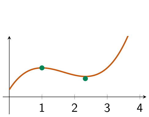
Antiderivatives and Indefinite Integrals

• Definition of Antiderivative: Given a function $f(x)$, an antiderivative of $f(x)$ is a function $F(x)$ such that $F'(x) = f(x)$.
  • Example: Since $\frac{d}{dx}(x^5) = 5x^4$, an antiderivative of $5x^4$ is $x^5$.
• Indefinite Integral Notation: If $F'(x) = f(x)$, then $\int f(x)\,dx = F(x) + C$.
• Role of the Arbitrary Constant $C$: The constant $C$ records all possible antiderivatives of $f(x)$. It is not a decorative symbol; because the derivative of any constant is zero, $\frac{d}{dx}(F(x) + C) = F'(x) + 0 = f(x)$.
• Uniqueness Up to a Constant: Suppose $F'(x) = G'(x)$ on an interval. Then $\frac{d}{dx}(F(x) - G(x)) = 0$. By the Mean Value Theorem, $F(x) - G(x) = C$ for some constant $C$. Consequently, on an interval, all antiderivatives of a given function differ by a constant.
• Visual Interpretation: Integration operates as the inverse process of differentiation.

• Linearity Rules: Antiderivatives satisfy linearity properties:
  • $\int (a f(x) + b g(x))\,dx = a \int f(x)\,dx + b \int g(x)\,dx$
  • Example: $\int (6x^2 - 4x + 7)\,dx = 2x^3 - 2x^2 + 7x + C$
• Power Rule for Antiderivatives: For any real exponent $n \neq -1$:
  • $\int x^n\,dx = \frac{x^{n+1}}{n+1} + C$
  • Example 1: $\int x^7\,dx = \frac{x^8}{8} + C$
  • Example 2: $\int \sqrt{x}\,dx = \int x^{1/2}\,dx = \frac{2}{3}x^{3/2} + C$
• The Exceptional Power $n = -1$: The standard power rule fails when $n = -1$ because it produces division by zero. Instead:
  • $\int \frac{1}{x}\,dx = \ln(|x|) + C$
  • Reason: $\frac{d}{dx}\ln(|x|) = \frac{1}{x}$ for all $x \neq 0$
• Fundamental Table of Exponential and Logarithmic Antiderivatives:
  • $\int e^x\,dx = e^x + C$
  • $\int a^x\,dx = \frac{a^x}{\ln(a)} + C$ for $a > 0, a \neq 1$
  • $\int \frac{1}{x}\,dx = \ln(|x|) + C$
  • $\int \frac{u'(x)}{u(x)}\,dx = \ln(|u(x)|) + C$
• Fundamental Table of Trigonometric Antiderivatives:
  • $\int \cos(x)\,dx = \sin(x) + C$
  • $\int \sin(x)\,dx = -\cos(x) + C$
  • $\int \sec^2(x)\,dx = \tan(x) + C$
  • $\int \csc^2(x)\,dx = -\cot(x) + C$
  • $\int \sec(x)\tan(x)\,dx = \sec(x) + C$
  • $\int \csc(x)\cot(x)\,dx = -\csc(x) + C$
• Inverse Trigonometric Antiderivatives:
  • $\int \frac{dx}{1 + x^2} = \arctan(x) + C$
  • $\int \frac{dx}{\sqrt{1 - x^2}} = \arcsin(x) + C$
  • General Form: $\int \frac{dx}{a^2 + x^2} = \frac{1}{a}\arctan\left(\frac{x}{a}\right) + C$ for $a > 0$
• Basic Integration Examples:
  • $\int \left(4x^3 - \frac{3}{x} + 5e^x\right)\,dx = x^4 - 3\ln(|x|) + 5e^x + C$
  • $\int \left(2\cos(x) - 7\sec^2(x)\right)\,dx = 2\sin(x) - 7\tan(x) + C$
• Verification Habit: The fastest method to detect integration errors is differentiating the anti-derivative result:
  • $\frac{d}{dx}\left(\frac{2}{3}x^{3/2} + C\right) = \frac{2}{3}\cdot\frac{3}{2}x^{1/2} + 0 = x^{1/2} = \sqrt{x}$

The Substitution Method for Integration

• Theoretical Principle: The substitution rule reverses the chain rule of differentiation. If $u = g(x)$, then $du = g'(x)\,dx$, transforming the integral:
  • $\int f(g(x))g'(x)\,dx = \int f(u)\,du$
  • After computing the antiderivative in terms of $u$, substitute back $u = g(x)$.
• Guidelines for Choosing $u$:
  1. An expression situated inside a power, radical, exponential, logarithm, or trigonometric function.
  2. A denominator whose derivative (up to a constant multiple) appears in the numerator.
  3. A complicated expression whose derivative almost appears in the integrand.
  • Warning: If $du$ does not match the remaining algebraic factors, substitution will not resolve the integral.
• Direct Substitution Example: Evaluate $\int 2x\cos(x^2 + 1)\,dx$
  • Let $u = x^2 + 1$, then $du = 2x\,dx$
  • $\int \cos(u)\,du = \sin(u) + C = \sin(x^2 + 1) + C$
• Constant Adjustment Example: Evaluate $\int x\sqrt{x^2 + 4}\,dx$
  • Let $u = x^2 + 4$, then $du = 2x\,dx \implies x\,dx = \frac{1}{2}du$
  • $\frac{1}{2}\int u^{1/2}\,du = \frac{1}{2}\cdot\frac{2}{3}u^{3/2} + C = \frac{1}{3}(x^2 + 4)^{3/2} + C$
• Logarithmic Form Example: Evaluate $\int \frac{3x^2}{x^3 + 5}\,dx$
  • Let $u = x^3 + 5$, then $du = 3x^2\,dx$
  • $\int \frac{du}{u} = \ln(|u|) + C = \ln(|x^3 + 5|) + C$
• Definite Integrals by Substitution: When evaluating a definite integral via substitution, the integration limits must be converted to the variable $u$:
  • $\int_a^b f(g(x))g'(x)\,dx = \int_{g(a)}^{g(b)} f(u)\,du$
  • Safe Method 1: Convert limits to $u$ and evaluate entirely in terms of $u$.
  • Safe Method 2: Find the antiderivative in terms of $x$ and evaluate using original limits $a$ and $b$
• Definite Integral Example: Evaluate $\int_0^2 x\sqrt{x^2 + 1}\,dx$
  • Let $u = x^2 + 1$, $du = 2x\,dx \implies x\,dx = \frac{1}{2}du$
  • Convert limits: When $x = 0$, $u = 0^2 + 1 = 1$. When $x = 2$, $u = 2^2 + 1 = 5$
  • $\frac{1}{2}\int_1^5 u^{1/2}\,du = \frac{1}{2}\left[\frac{2}{3}u^{3/2}\right]_1^5 = \frac{1}{3}\left(5^{3/2} - 1^{3/2}\right) = \frac{5\sqrt{5} - 1}{3}$
• Mixed Variables Error: A $u$-integral must never retain remaining factors of $x$. For example, transforming $\int x\sqrt{x^2 + 4}\,dx$ into $\int x\sqrt{u}\,du$ is mathematically invalid.

Advanced and Challenging Integration Techniques

• Root Substitution Technique: Evaluate $\int \frac{e^{2x}}{\sqrt[4]{e^x + 1}}\,dx$
  • Set $e^x + 1 = t^4 \implies e^x = t^4 - 1$ and $e^{2x} = (t^4 - 1)^2$
  • Differentiate $e^x + 1 = t^4$ to get $e^x\,dx = 4t^3\,dt \implies dx = \frac{4t^3}{e^x}\,dt = \frac{4t^3}{t^4 - 1}\,dt$
  • Substitute into integral: $\int \frac{(t^4 - 1)^2}{t}\cdot\frac{4t^3}{t^4 - 1}\,dt = 4\int t^2(t^4 - 1)\,dt = 4\int (t^6 - t^2)\,dt$
  • Integrate: $4\left(\frac{t^7}{7} - \frac{t^3}{3}\right) + C = \frac{4}{7}t^7 - \frac{4}{3}t^3 + C$
  • Substitute back $t = (e^x + 1)^{1/4}$:
  • $\frac{4}{7}(e^x + 1)^{7/4} - \frac{4}{3}(e^x + 1)^{3/4} + C$
• Trigonometric-Rational Integral: Evaluate $\int \frac{dx}{2\cos^2(x) + 5\sin^2(x)}$
  • Set $t = \tan(x) \implies dt = \sec^2(x)\,dx = (1 + t^2)\,dx \implies dx = \frac{dt}{1 + t^2}$
  • Express trigonometric powers in terms of $t$:
    • $\cos^2(x) = \frac{1}{1 + t^2}$
    • $\sin^2(x) = \frac{t^2}{1 + t^2}$
  • Rewrite denominator: $2\cos^2(x) + 5\sin^2(x) = \frac{2 + 5t^2}{1 + t^2}$
  • Substitute: $\int \frac{\frac{dt}{1 + t^2}}{\frac{2 + 5t^2}{1 + t^2}} = \int \frac{dt}{2 + 5t^2} = \frac{1}{2}\int \frac{dt}{1 + \left(\sqrt{\frac{5}{2}}t\right)^2}$
  • Integrate: $\frac{1}{2}\cdot\frac{1}{\sqrt{\frac{5}{2}}}\arctan\left(\sqrt{\frac{5}{2}}t\right) + C = \frac{1}{\sqrt{10}}\arctan\left(\sqrt{\frac{5}{2}}t\right) + C$
  • Substitute back $t = \tan(x)$: $\frac{1}{\sqrt{10}}\arctan\left(\sqrt{\frac{5}{2}}\tan(x)\right) + C$
• Algebraic Power-Root Integral: Evaluate $\int \frac{x^7}{\sqrt[4]{1 + x^2}}\,dx$
  • Let $1 + x^2 = t^4 \implies x^2 = t^4 - 1$ and $2x\,dx = 4t^3\,dt \implies x\,dx = 2t^3\,dt$
  • Decompose numerator: $x^7\,dx = (x^2)^3(x\,dx) = (t^4 - 1)^3 (2t^3\,dt)$
  • Substitute: $\int \frac{(t^4 - 1)^3\cdot 2t^3\,dt}{t} = 2\int t^2(t^4 - 1)^3\,dt$
  • Expand $(t^4 - 1)^3 = t^{12} - 3t^8 + 3t^4 - 1$:
    • $2\int t^2(t^{12} - 3t^8 + 3t^4 - 1)\,dt = 2\int (t^{14} - 3t^{10} + 3t^6 - t^2)\,dt$
  • Integrate: $2\left(\frac{t^{15}}{15} - \frac{3t^{11}}{11} + \frac{3t^7}{7} - \frac{t^3}{3}\right) + C$
  • Substitute back $t = (1 + x^2)^{1/4}$.
  • $\frac{2}{15}(1 + x^2)^{15/4} - \frac{6}{11}(1 + x^2)^{11/4} + \frac{6}{7}(1 + x^2)^{7/4} - \frac{2}{3}(1 + x^2)^{3/4} + C$
• Logarithmic-Root Integral: Evaluate $\int \frac{(\ln(x))^2}{x\sqrt[3]{2 + \ln(x)}}\,dx$ for $x > e^{-2}$
  • Set $2 + \ln(x) = t^3 \implies \ln(x) = t^3 - 2$ and $\frac{dx}{x} = 3t^2\,dt$
  • Substitute: $\int \frac{(t^3 - 2)^2}{t}\cdot 3t^2\,dt = 3\int t(t^3 - 2)^2\,dt = 3\int t(t^6 - 4t^3 + 4)\,dt = 3\int (t^7 - 4t^4 + 4t)\,dt$
  • Integrate: $3\left(\frac{t^8}{8} - \frac{4t^5}{5} + 2t^2\right) + C = \frac{3}{8}t^8 - \frac{12}{5}t^5 + 6t^2 + C$
  • Substitute back $t = (2 + \ln(x))^{1/3}$.
  • $\frac{3}{8}(2 + \ln(x))^{8/3} - \frac{12}{5}(2 + \ln(x))^{5/3} + 6(2 + \ln(x))^{2/3} + C$
• Radicand Denominator Integral: Evaluate $\int \frac{x^3}{\sqrt{x^2 + 1} + 1}\,dx$
  • Set $u = \sqrt{x^2 + 1} + 1 \implies u - 1 = \sqrt{x^2 + 1} \implies (u - 1)^2 = x^2 + 1 \implies x^2 = u^2 - 2u$
  • Differentiate $x^2 = u^2 - 2u \implies 2x\,dx = (2u - 2)\,du \implies x\,dx = (u - 1)\,du$
  • Decompose $x^3\,dx = x^2(x\,dx) = (u^2 - 2u)(u - 1)\,du$
  • Substitute: $\int \frac{(u^2 - 2u)(u - 1)}{u}\,du = \int (u - 2)(u - 1)\,du = \int (u^2 - 3u + 2)\,du$
  • Integrate: $\frac{u^3}{3} - \frac{3u^2}{2} + 2u + C$
  • Substitute back $u = \sqrt{x^2 + 1} + 1$
  • $\frac{(\sqrt{x^2 + 1} + 1)^3}{3} - \frac{3(\sqrt{x^2 + 1} + 1)^2}{2} + 2(\sqrt{x^2 + 1} + 1) + C$
• Rational Quadratic Square Integral: Evaluate $\int \frac{x^3}{(x^2 + 2x + 2)^2}\,dx$
  • Complete the square: $x^2 + 2x + 2 = (x + 1)^2 + 1$
  • Set $u = x + 1 \implies x = u - 1, dx = du, x^2 + 2x + 2 = u^2 + 1$
  • Expand numerator: $(u - 1)^3 = u^3 - 3u^2 + 3u - 1$
  • Rewrite integral: $\int \frac{u^3 - 3u^2 + 3u - 1}{(u^2 + 1)^2}\,du$
  • Split into partial fractions:
    • $\int \frac{u^3}{(u^2 + 1)^2}\,du = \frac{1}{2}\ln(u^2 + 1) + \frac{1}{2(u^2 + 1)}$
    • $\int \frac{-3u^2}{(u^2 + 1)^2}\,du = -3\left(\frac{1}{2}\arctan(u) - \frac{u}{2(u^2 + 1)}\right)$
    • $\int \frac{3u}{(u^2 + 1)^2}\,du = -\frac{3}{2(u^2 + 1)}$
    • $\int \frac{-1}{(u^2 + 1)^2}\,du = -\frac{1}{2}\arctan(u) - \frac{u}{2(u^2 + 1)}$
  • Combine and simplify in variable $u$:
    • $\frac{1}{2}\ln(u^2 + 1) - \frac{3}{2}\arctan(u) - \frac{u^2 + 3u - 1}{2(u^2 + 1)} + C$
  • Substitute back $u = x + 1$
  • $\frac{1}{2}\ln(x^2 + 2x + 2) - \frac{3}{2}\arctan(x + 1) - \frac{(x + 1)^2 + 3(x + 1) - 1}{2(x^2 + 2x + 2)} + C$

The Extreme Value Theorem and Absolute Extrema

• Local vs. Absolute Extrema:
  • Local Maximum/Minimum: A point where the function value is the highest or lowest relative to immediately surrounding points.
  • Absolute Maximum/Minimum: The overall highest or lowest output value across the function's entire domain.
  • On a closed interval, boundaries (endpoints) matter as much as interior critical points.

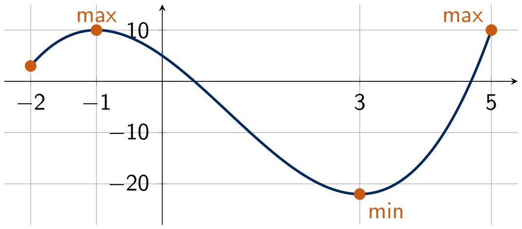
• Extreme Value Theorem (EVT): If $f$ is continuous on a closed interval $[a, b]$, then $f$ attains both an absolute maximum and an absolute minimum on $[a, b]$.
  • Formal Statement: There exist points $c, d \in [a, b]$ such that $f(c) \le f(x) \le f(d)$ for every $x \in [a, b]$.
• Necessity of Hypotheses:
  • Non-Closed Interval: The function $f(x) = x$ on $(0, 1)$ has no absolute minimum or maximum because the endpoint boundaries $0$ and $1$ are excluded.
  • Discontinuity: The piecewise function $f(x) = x$ for $0 \le x < 1$ and $f(1) = 0$ on $[0, 1]$ lacks an absolute maximum because its values approach $1$ without ever reaching it.
• The Closed Interval Method: To find absolute extrema of a continuous function $f$ on $[a, b]$:
  1. Verify that $f$ is continuous on $[a, b]$.
  2. Find all critical numbers of $f$ in the open interval $(a, b)$ where $f'(x) = 0$ or $f'(x)$ does not exist.
  3. Evaluate $f(x)$ at every critical number and at the endpoints $a$ and $b$
  4. Compare all resulting values. The maximum output is the absolute maximum; the minimum output is the absolute minimum.
• EVT Example 1 (Polynomial): Find absolute extrema of $f(x) = x^3 - 3x^2 - 9x + 5$ on $[-2, 5]$
  • Compute derivative: $f'(x) = 3x^2 - 6x - 9 = 3(x - 3)(x + 1)$
  • Critical numbers in $(-2, 5)$: $x = -1, 3$
  • Evaluate inputs:
    • $f(-2) = (-2)^3 - 3(-2)^2 - 9(-2) + 5 = 3$
    • $f(-1) = (-1)^3 - 3(-1)^2 - 9(-1) + 5 = 10$
    • $f(3) = (3)^3 - 3(3)^2 - 9(3) + 5 = -22$
    • $f(5) = (5)^3 - 3(5)^2 - 9(5) + 5 = 10$
  • Conclusion: Absolute maximum value is $10$ at $x = -1$ and $x = 5$. Absolute minimum value is $-22$ at $x = 3$.

• EVT Example 2 (Trigonometric Function): Find absolute extrema of $f(x) = \sin(x) + \cos(x)$ on $[0, \pi]$
  • Compute derivative: $f'(x) = \cos(x) - \sin(x) = 0 \implies \tan(x) = 1$
  • Critical number in $[0, \pi]$: $x = \pi/4$
  • Evaluate inputs: $f(0) = 1$, $f(\pi/4) = \sqrt{2}$, $f(\pi) = -1$
  • Conclusion: Absolute maximum is $\sqrt{2}$ at $x = \pi/4$. Absolute minimum is $-1$ at $x = \pi$.
• EVT Example 3 (Radical Function): Find absolute extrema of $f(x) = \sqrt{x}(4 - x)$ on $[0, 4]$
  • Compute derivative for $x > 0$: $f'(x) = \frac{1}{2\sqrt{x}}(4 - x) - \sqrt{x} = \frac{4 - 3x}{2\sqrt{x}}$
  • Critical numbers: $x = 4/3$ (where $f' = 0$) and $x = 0$ (endpoint where $f'$ is undefined)
  • Evaluate inputs: $f(0) = 0$, $f(4/3) = \sqrt{4/3}(4 - 4/3) = \frac{16}{3\sqrt{3}}$, $f(4) = 0$
  • Conclusion: Absolute maximum is $\frac{16}{3\sqrt{3}}$ at $x = 4/3$. Absolute minimum is $0$ at $x = 0$ and $x = 4$
• EVT Example 4 (Rational Function): Find absolute extrema of $f(x) = \frac{x}{x^2 + 1}$ on $[-2, 2]$
  • Compute derivative: $f'(x) = \frac{(x^2 + 1) - 2x^2}{(x^2 + 1)^2} = \frac{1 - x^2}{(x^2 + 1)^2}$
  • Critical numbers: $x = \pm 1$
  • Evaluate inputs: $f(-2) = -2/5$, $f(-1) = -1/2$, $f(1) = 1/2$, $f(2) = 2/5$
  • Conclusion: Absolute maximum is $1/2$ at $x = 1$. Absolute minimum is $-1/2$ at $x = -1$.
• EVT Example 5 (Exponential Function): Find absolute extrema of $f(x) = xe^{-x}$ on $[0, 4]$
  • Compute derivative: $f'(x) = e^{-x} - xe^{-x} = e^{-x}(1 - x)$
  • Critical number: $x = 1$
  • Evaluate inputs: $f(0) = 0$, $f(1) = 1/e$, $f(4) = 4/e^4$
  • Conclusion: Absolute maximum is $1/e$ at $x = 1$. Absolute minimum is $0$ at $x = 0$
• EVT Example 6 (Logarithmic Function): Find absolute extrema of $f(x) = \ln(x) - x$ on $[1/2, 4]$
  • Compute derivative: $f'(x) = \frac{1}{x} - 1 = \frac{1 - x}{x}$
  • Critical number: $x = 1$
  • Evaluate inputs: $f(1/2) = -\ln(2) - 1/2 \approx -1.193$, $f(1) = -1$, $f(4) = \ln(4) - 4 \approx -2.614$
  • Conclusion: Absolute maximum is $-1$ at $x = 1$. Absolute minimum is $\ln(4) - 4$ at $x = 4$

Logarithmic Differentiation and Derivative Sign Analysis

• Scope of Application: Logarithmic differentiation is indicated for functions involving complex products, multi-term quotients, fractional exponents, and variable powers ($y = u(x)^{v(x)}$).
• Standard Procedure:
  1. Take the natural logarithm of both sides: $\ln(y) = \ln(f(x))$
  2. Simplify the right side using logarithm expansion rules: $\ln(AB) = \ln(A) + \ln(B)$, $\ln(A/B) = \ln(A) - \ln(B)$, $\ln(A^r) = r\ln(A)$.
  3. Differentiate implicitly with respect to $x$: $\frac{y'}{y} = \frac{d}{dx}[\ln(f(x))]$
  4. Solve for $y'$: $y' = y \cdot \frac{d}{dx}[\ln(f(x))]$
  5. Substitute the original expression for $y$
• Logarithmic Differentiation Examples:
  • Variable Power $y = x^x$ ($x > 0$):
    • $\ln(y) = x\ln(x) \implies \frac{y'}{y} = \ln(x) + 1 \implies y' = x^x(\ln(x) + 1)$
  • Trigonometric Power $y = (\sin(x))^x$ ($\sin(x) > 0$):
    • $\ln(y) = x\ln(\sin(x)) \implies \frac{y'}{y} = \ln(\sin(x)) + x\cot(x) \implies y' = (\sin(x))^x [\ln(\sin(x)) + x\cot(x)]$
  • Product of Powers $y = (x^2 + 1)^5(3x - 1)^4\sqrt{x + 2}$:
    • $\ln(y) = 5\ln(x^2 + 1) + 4\ln(3x - 1) + \frac{1}{2}\ln(x + 2)$
    • $\frac{y'}{y} = \frac{10x}{x^2 + 1} + \frac{12}{3x - 1} + \frac{1}{2(x + 2)}$
    • $y' = (x^2 + 1)^5(3x - 1)^4\sqrt{x + 2} \left[\frac{10x}{x^2 + 1} + \frac{12}{3x - 1} + \frac{1}{2(x + 2)}\right]$
  • Complex Quotient $y = \frac{x^3\sqrt{x^2 + 4}}{(5x - 2)^7(x + 1)^2}$:
    • $\ln(y) = 3\ln(x) + \frac{1}{2}\ln(x^2 + 4) - 7\ln(5x - 2) - 2\ln(x + 1)$
    • $\frac{y'}{y} = \frac{3}{x} + \frac{x}{x^2 + 4} - \frac{35}{5x - 2} - \frac{2}{x + 1}$
    • $y' = y \left[\frac{3}{x} + \frac{x}{x^2 + 4} - \frac{35}{5x - 2} - \frac{2}{x + 1}\right]$
  • Variable Radical Power $y = (\ln(x))^{\sqrt{x}}$ ($x > 1$):
    • $\ln(y) = \sqrt{x}\ln(\ln(x))$
    • $\frac{y'}{y} = \frac{1}{2\sqrt{x}}\ln(\ln(x)) + \sqrt{x}\cdot\frac{1}{x\ln(x)} = \frac{\ln(\ln(x))}{2\sqrt{x}} + \frac{1}{\sqrt{x}\ln(x)}$
    • $y' = (\ln(x))^{\sqrt{x}} \left[\frac{\ln(\ln(x))}{2\sqrt{x}} + \frac{1}{\sqrt{x}\ln(x)}\right]$
  • Exponential Base Power $y = (x^2 + 1)^{\sin(x)}$:
    • $\ln(y) = \sin(x)\ln(x^2 + 1)$
    • $\frac{y'}{y} = \cos(x)\ln(x^2 + 1) + \sin(x)\cdot\frac{2x}{x^2 + 1}$
    • $y' = (x^2 + 1)^{\sin(x)} \left[\cos(x)\ln(x^2 + 1) + \frac{2x\sin(x)}{x^2 + 1}\right]$
• Monotonicity Analysis via $\frac{f'}{f}$: If $f(x) > 0$, then $f'(x) = f(x)\frac{d}{dx}[\ln(f(x))]$. Since $f(x) > 0$, the sign of $f'(x)$ is completely determined by the sign of $\frac{f'(x)}{f(x)} = \frac{d}{dx}[\ln(f(x))]$.
  • Example 1: $f(x) = \frac{x}{x^2 + 1}$ for $x > 0$
    • $\ln(f) = \ln(x) - \ln(x^2 + 1) \implies \frac{f'}{f} = \frac{1}{x} - \frac{2x}{x^2 + 1} = \frac{1 - x^2}{x(x^2 + 1)}$
    • The sign depends on $1 - x^2$. Thus, $f$ is increasing on $(0, 1)$ and decreasing on $(1, \infty)$.
  • Example 2: $f(x) = x^2 e^{-x}$ for $x > 0$
    • $\ln(f) = 2\ln(x) - x \implies \frac{f'}{f} = \frac{2}{x} - 1 = \frac{2 - x}{x}$
    • $f$ is increasing on $(0, 2)$ and decreasing on $(2, \infty)$.
  • Example 3: $f(x) = \frac{x^3}{(x + 1)^4}$ for $x > 0$
    • $\ln(f) = 3\ln(x) - 4\ln(x + 1) \implies \frac{f'}{f} = \frac{3}{x} - \frac{4}{x + 1} = \frac{3 - x}{x(x + 1)}$
    • $f$ is increasing on $(0, 3)$ and decreasing on $(3, \infty)$.
  • Example 4: $f(x) = x^a(1 - x)^b$ for $0 < x < 1$ ($a, b > 0$)
    • $\ln(f) = a\ln(x) + b\ln(1 - x) \implies \frac{f'}{f} = \frac{a}{x} - \frac{b}{1 - x} = \frac{a - (a + b)x}{x(1 - x)}$
    • $f$ is increasing on $\left(0, \frac{a}{a + b}\right)$ and decreasing on $\left(\frac{a}{a + b}, 1\right)$.

The Intermediate Value Theorem and Numerical Root Finding

• Intermediate Value Theorem (IVT): If $f$ is continuous on $[a, b]$ and $N$ is any real number between $f(a)$ and $f(b)$, then there exists at least one value $c \in (a, b)$ such that f(c) = N$.\n * *Root-Finding Variant*: If f$is continuous on$[a, b]$and$f(a)f(b) < 0$(opposite signs), there exists$c \in (a, b)$such that$f(c) = 0$.
• IVT Application Examples:
  • Polynomial Root: Show $f(x) = x^3 + x - 1$ has a root in $(0, 1)$.
    • $f(0) = -1 < 0$ and $f(1) = 1 > 0$. By IVT, a root $c \in (0, 1)$ exists.
  • Trigonometric Root: Show $f(x) = \cos(x) - x$ has a root in $(0, 1)$.
    • $f(0) = 1 > 0$ and $f(1) = \cos(1) - 1 < 0$. By IVT, $\cos(c) = c$ for some $c \in (0, 1)$.
  • Logarithmic Equation: Show $\ln(x) = x - 2$ has a solution in $(1, 4)$.
    • Define $f(x) = \ln(x) - x + 2$. $f(1) = 1 > 0$ and $f(4) = \ln(4) - 2 \approx -0.614 < 0$. IVT guarantees a root.
  • Sequential Sign Testing: For $f(x) = x^3 - 2x - 5$:
    • $f(2) = -1 < 0$ and $f(3) = 16 > 0 \implies$ root lies in $(2, 3)$.
    • Midpoint $x = 2.5$: $f(2.5) = 5.625 > 0 \implies$ root lies in $(2, 2.5)$.
    • Midpoint $x = 2.25$: $f(2.25) = 1.890625 > 0 \implies$ root lies in $(2, 2.25)$.
• Bisection Method Procedure:
  1. Start with an interval $[a, b]$ where $f(a)f(b) < 0$
  2. Calculate the midpoint $m = \frac{a + b}{2}$
  3. If $f(m) = 0$, $m$ is the exact root.
  4. If $f(a)f(m) < 0$, the root lies in $[a, m]$. Set new interval to $[a, m]$.
  5. If $f(m)f(b) < 0$, the root lies in $[m, b]$. Set new interval to $[m, b]$.
  6. Repeat sequentially. Each step halves the interval length.
• Bisection Error Analysis:
  • After $n$ bisection steps, the interval length is $\frac{b - a}{2^n}$.
  • The maximum error when estimating the root by the midpoint of the final interval is $\frac{b - a}{2^{n + 1}}$.
  • Step Calculation Example: To guarantee interval length below $\varepsilon = 0.001$ starting from $[2, 3]$:
    • $\frac{1}{2^n} < 0.001 \implies 2^n > 1000$. Since $2^{10} = 1024$, $10$ bisection steps are required.
• Bisection Worked Example 1 ($x^3 + x - 1 = 0$ on $[0, 1]$):
  • Initial: $f(0) = -1$, $f(1) = 1$
  • Step 1: $m_1 = 0.5$, $f(0.5) = -0.375 < 0 \implies$ interval $[0.5, 1]$
  • Step 2: $m_2 = 0.75$, $f(0.75) = 0.171875 > 0 \implies$ interval $[0.5, 0.75]$
  • Step 3: $m_3 = 0.625$, $f(0.625) = -0.130859 < 0 \implies$ interval $[0.625, 0.75]$
  • Step 4: $m_4 = 0.6875$, $f(0.6875) \approx 0.01245 > 0 \implies$ interval $[0.625, 0.6875]$
  • Midpoint estimate: $x \approx \frac{0.625 + 0.6875}{2} = 0.65625$
• Bisection Worked Example 2 ($\cos(x) = x$ on $[0, 1]$):
  • Initial: $f(0) = 1 > 0$, $f(1) = \cos(1) - 1 < 0$
  • Step 1: $m_1 = 0.5$, $f(0.5) = \cos(0.5) - 0.5 \approx 0.3776 > 0 \implies$ interval $[0.5, 1]$
  • Step 2: $m_2 = 0.75$, $f(0.75) = \cos(0.75) - 0.75 \approx -0.0183 < 0 \implies$ interval $[0.5, 0.75]$