Constant Multiple Rule: g(x)=cf(x) then g’(x)=cf’(x)
Power Rule: f(x)=xn then f’(x)=nxn−1
Sum and Difference Rule: h(x)=f(x)±g(x) thenh’(x)=f’(x)±g’(x)
Product Rule (also applies to cross and dot products): h(x)=f(x)g(x) then h’(x)=f’(x)g(x)+f(x)g’(x)
Quotient Rule: h(x)=g(x)f(x) then h’(x)=g(x)2f’(x)g(x)−f(x)g’(x)
Chain Rule: h(x)=f(g(x)) then h’(x)=f’(g(x))g’(x)
Trig Derivatives:
f(x)=sin(x) then f’(x)=cos(x)
f(x)=cos(x) then f’(x)=−sin(x)
f(x)=tan(x) then f’(x)=sec2(x)
f(x)=sec(x) then f’(x)=sec(x)tan(x)
f(x)=cot(x) then f’(x)=−csc2(x)
f(x)=csc(x) then f’(x)=−csc(x)cot(x)
Exponential and Logarithmic Derivatives
f(x)=ax then f’(x)=ln(a)ax
f(x)=ex then f’(x)=ex
f(x)=loga(x) then f’(x)=ln(a)x1
f(x)=ln(x) then f’(x)=x1
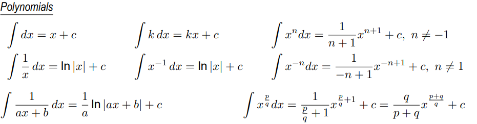
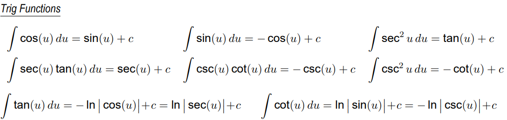
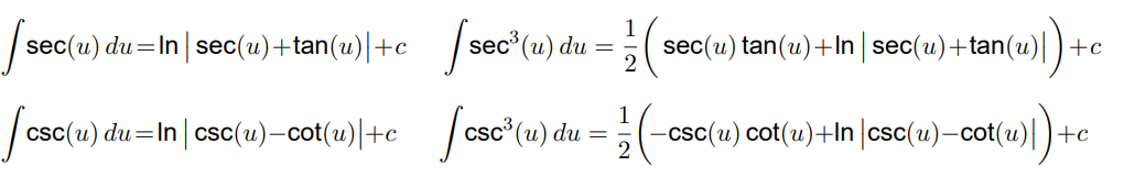
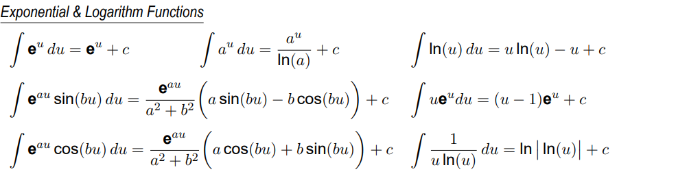
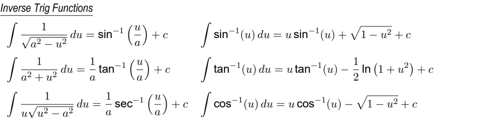
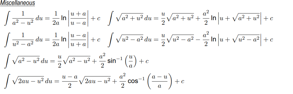
Integrals
Integrations by Parts:∫udv=uv−∫vdu
Formulas
If r(t)=f(t)i+g(t)j+h(t)k , then r’(t)=f’(t)i+g’(t)j+h’(t)k
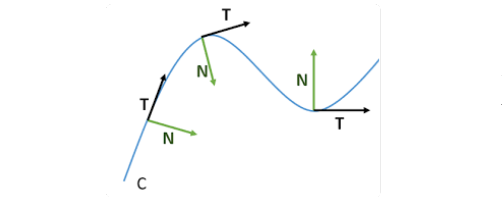
The Unit Tangent Vector is a vector with the length of 1 and goes the same direction as r(a).
T(t)=∣r’(t)∣r’(t)
Another important measurement is how the unit tangent vector is changing directions, which is represented via the Principal Unit Normal Vector, which can be calculated via the following formula:
N(s)=∣dT/ds∣dT/ds=κ1dsdT
A special aspect of the Principal Unit Normal Vector is that it is always orthogonal to the Unit Tangent Vector
Position, Velocity, Speed, and Acceleration still have the same relationship, where Position is r(t), Velocity is v(t)=r’(t) , Speed is ∣v(t)∣, and Acceleration is a
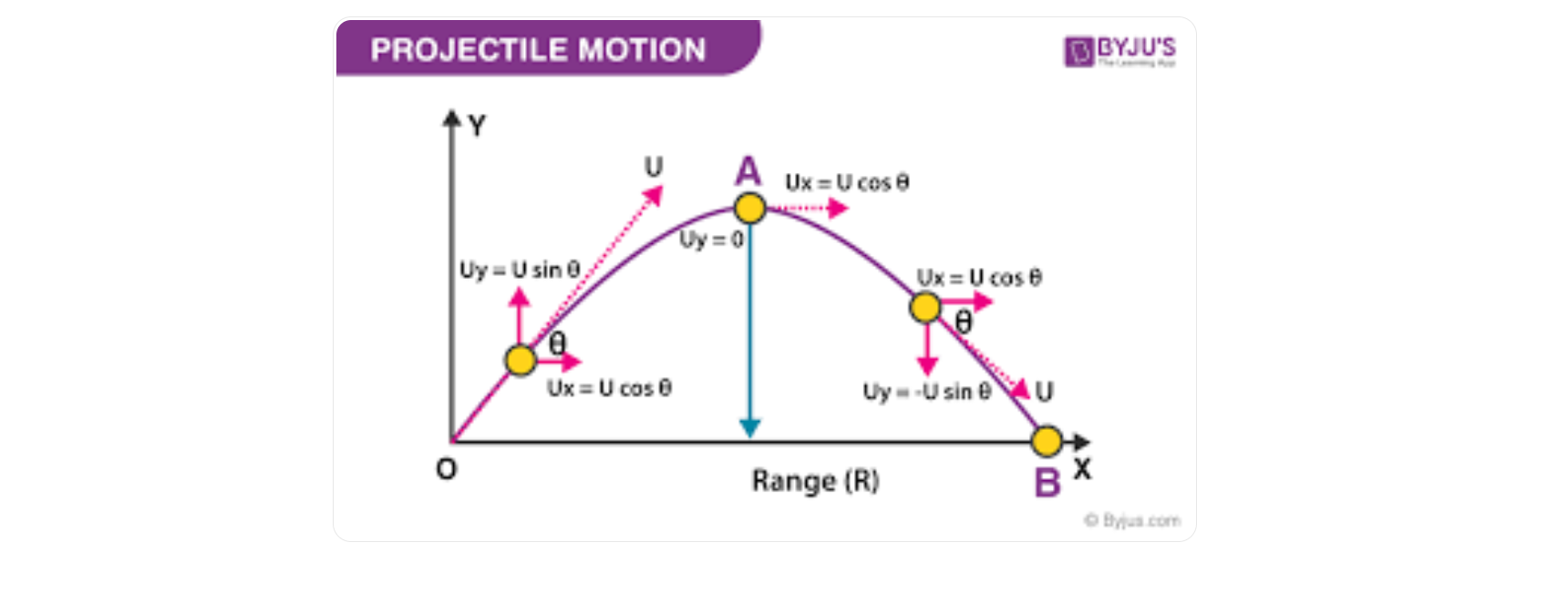
When given physics problems that relates to throwing something, the x and z components are usually either constant or have a constant acceleration affecting them. On the other hand, the y component will be affected by both their initial position and gravity. Because of this the following equations are true:
Based off a few kinematic equations, you can derive the following important properties of the parabolic arc:
time of flight =T=g2∣v0∣sin(α)
range =g∣v0∣2sin(2α)
maximum height =y(2T)=2g(∣v0∣sin(α))2
Another topic we have previously covered in Calculus BC is arc length, which tells the length of a curve should it have been stretched out into a straight line. It is calculated via the following formula:
∫abf’(t)2+g’(t)2+h’(t)2dt=∫ab∣r’(t)∣dt
When you have to make arc length a function of a parameter, use the following variation of the formula:
s(t)=∫at∣v(u)∣du
Curvature describes how fast the direction is changing, which can be described with the following formulas
κ=∣v∣1∣dtdT∣=∣r’(t)∣∣T’(t)∣=∣v∣3∣v×a∣ where T is the unit tangent vector, v is the velocity vector, and a is the acceleration vector
The acceleration vector also has some tangential properties, mainly the following:
a=aNN+aTT whereaN=κ∣v∣2=v∣v×a∣ and aT=dt2d2s=∣v∣v⋅a.
The Unit Binormal Vector is the vector which represents the direction by which a point exits a plane made by the T and N vectors via Torsion