Econ 101
macro vs micro
microeconomics - how households/business make choices
macroeconomics - how individuals, firms/markets, or economy function together
4 core principles of economics
opportunity cost principle - choices have trade offs
opportunity cost - value of next best alternative
part of true cost
ex. college vs getting a job
cost benefit principle - benefits should be greater than costs
incentives shape decisions
associated w any choice
pursue IF benefits > cost
marginal principle - will one more be beneficial?
do until marg benefit = marg cost
interdependence principle - decisions are based on other decisions
yours, other people’s, market’s, etc
SUNK COSTS DO NOT MATTER
sunk cost - resources used that cannot be gotten back
Production possibilities frontier - shows max amount one can produce given resources/tech
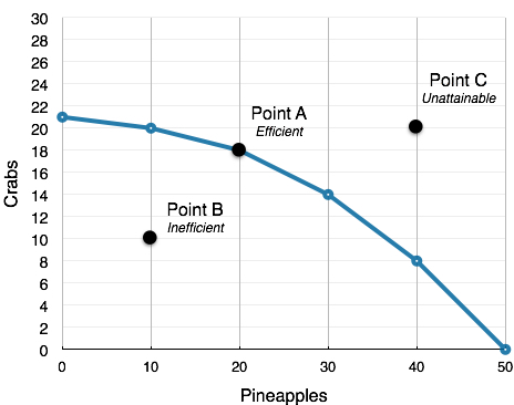
Points
on curve → efficient
inside curve → inefficient, but possible
outside curve → unattainable
Opportunity cost = slope
Shape
linear - constant opportunity cost
slope never changes
bowed out - increasing opportunity cost
slope is not constant
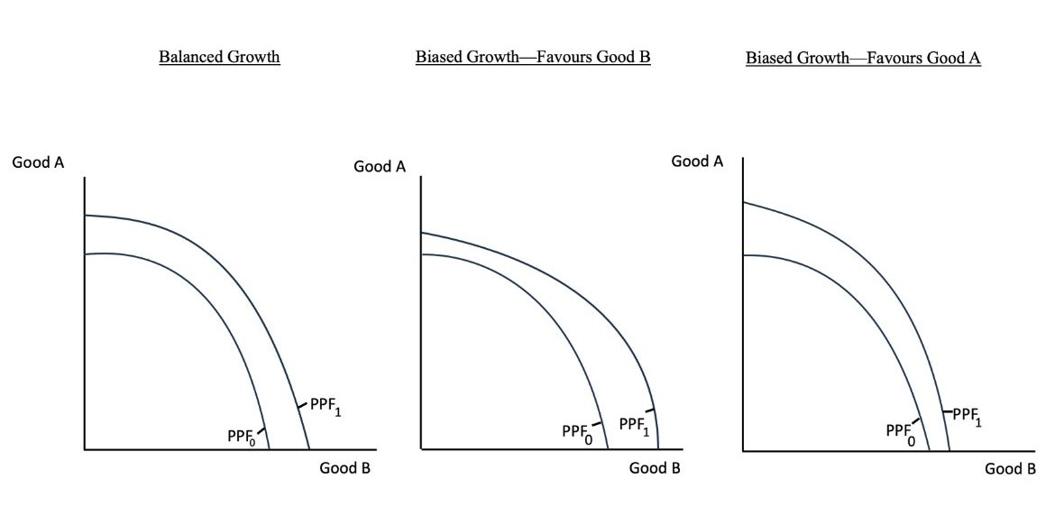
shifts
change in tech/resources (efficiency)
Trade advantage
absolute advantage - ability to produce more (or same) with same (or less) resources
comparative advantage - ability to produce good at lower opportunity cost
based on resource allocation
trade
comparative advantage in a good → specialize in production of good
set price btwn opportunity cost of goods
point should be outside the ppf
price
message to buyer/seller
incentive
bundle of info
allocates resources to more valuable area
Demand
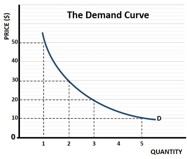
demand - relationship btwn price + quantity demanded
consumer
shown by demand schedule
quantity demanded - amount of a good/service consumers are willing/able to pay at a price
market demand - demand by all consumers of a given good/service
add up quantity demanded by individual for each respective price
law of demand - ceteris paribus, price increases → quantity demanded decreases
substitution effect
price increase → consumers shop for cheaper alternatives
income effect
price increase → consumers afford less w the same amount of money
Rational rule for buyers
how many? → one more? → Marg benefit vs price → consider alt → marg benefit ≥ price → buy
Demand = WTP = MB
WTP = willingness to pay
MB = marginal benefit
determinants of demand
income
income increase → demand increase
normal vs inferior goods
normal good - luxury stuff
ex. steak, new cars
income increase → demand increase
inferior good - cheap stuff
ex. cup noodles, used cars
income increase → demand decrease
price of related goods
demand complements - goods bought together
ex. hot dogs and buns
good 1 price increase → demand for good 1 decrease → demand for good 2 decrease
demand substitutes - alternatives
ex. pepsi and coke
good 1 price increase → demand for good 1 decrease → demand for good 2 increase
tastes/preferences
taste increase → demand increase
expectations
expected price increase in future → current demand increase
network effects
some goods more valuable when more people use it
ex. social media
more people have product → demand increase
congestion effects
some goods less valuable when more people use it
ex. amusement park
more people have product → demand decrease
number/type of consumers
more consumers → demand increase
CHANGE IN PRICE OF GOOD IS A MOVEMENT, NOT A SHIFT
Supply
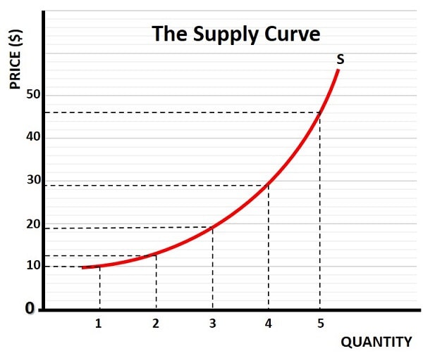
supply - relationship btwn price + quantity supplied
seller
shown by supply table
quantity supplied - amount of a good/service a firm is williing to supply at a price
market supply - supply by all firms/sellers of a given good/service
add up quantity supplied by seller for each respective price
law of supply - ceteris paribus, price increase → quantity supplied increases
Supply = MC
MC = marginal cost
firms sell at a price that is at least what it costs to produce a good/service
determinants of supply
price of inputs
price of inputs increase → supply decrease
technology/human capital changes
human capital - knowledge/skill of workers
productivity increase → marg costs decrease → supply increase
price of complements/substitutes
supply complements - goods produced together
ex. beef and leather
price of good 1 increase → supply of good 2 increase
supply substitutes - alternative goods a firm can produce w the same resources
ex. sun butter vs peanut butter
price of good 1 increase → supply of good 2 decrease
expectations
expected price increase in the future → current supply decrease
number/type of seller
more sellers → supply increases
CHANGE IN PRICE OF GOOD IS A MOVEMENT, NOT A SHIFT
equilibrium
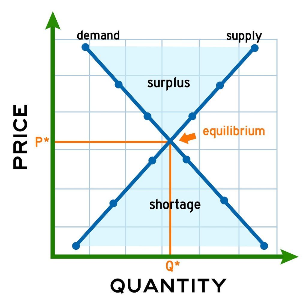
quantity demanded = quantity supplied
Demand + supply = market
how to find equilibrium
graphically - intersection
algebraically - set Qd = Qs
demand + supply schedules - find where Qd = Qs
Shortage and Supply
Shortage
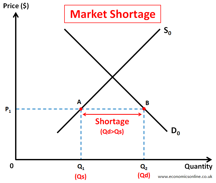
Quantity demanded > quantity supplied
upward pressure on price
excess demand
surplus
quantity demanded < quantity supplied
downward pressure on price
excess supply
the invisible hand - converging to equilibrium without direct govt intervention
value vs price
value - benefit ppl get from consuming a good/service
price - what ppl pay to consume a good/service
Surpluses
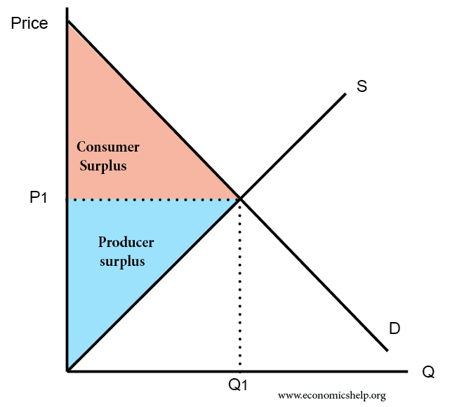
Consumer surplus
WTP - price or MB - price
area under the MB curve + above the price line
Producer surplus
price - MC
area under the price line + above the MC curve
Total/economic surplus
TS = PS + CS
Efficiency
rational rule of markets - produce good if MB ≥ MC
economic efficiency - MC = MB
economic surplus is maximized
market equilibrium
Dead weight loss - market is not efficient
DWL = TS (efficient) - TS (inefficient)
DWL = MB - MC
for all goods under/over produced relative to efficient quantity
Market failure - forces of supply/demand are inefficient → failure to produce efficient level of output
market power
externalities
private information
irrationality
govt regulations
Externality - benefit/cost that affects someone not directly involved with production/consumption of a good/service
private costs/benefits accrued to consumers/producers ≠ total costs/benefits accrued to society
marginal private cost (MPC) ≠ marginal social cost (MSC)
marginal private benefit (MPB) ≠ Marginal social benefit (MSB)
3rd parties affected → TS maximized when MSB = MSC
types of externalities
negative - generate external costs

MSC = MPC + MEC
MEC - marginal external cost
demand = MPB = MSB
supply - MPC
in production
ex. raising cattle → methane → climate change
in consumption
ex. use gasoline → greenhouse gases → climate change
overproduction
positive - generate external benefits
MSB = MPB + MEB
MEB - marginal external benefit
in production
ex. raising bees for honey → bees pollinate flowers
in consumption
ex. get a vaccine → one less person passing on flu → ppl protected
underproduction
evaluating policies
positive analysis - what IS happening, why, or predicitons
normative analysis - what SHOULD happen
value judgement
efficiency or equity
Elasticity

elasticity - responsiveness of one econ variable to a change in another econ variable
slope ≠ elasticity
Demand
how responsive quantity demanded is to change in price
USE ABSOLUTE VALUE
always negative bc of law of demand
Elastic - responsive
> 1
∆ quantity demanded > ∆ price
flatter curve → more elastic
inelastic - not responsive
< 1
∆ quantity demanded < ∆ price
unit elastic - 1:1 responsive
= 1
∆ quantity demanded = ∆ price
Supply
how responsive quantity supplied is to changes in price
Elastic - responsive
> 1
∆ quantity supplied > ∆ price
flatter curve → more elastic
inelastic - not responsive
< 1
∆ quantity supplied < ∆ price
unit elastic - 1:1 responsive
= 1
∆ quantity supplied = ∆ price
Perfectly elastic
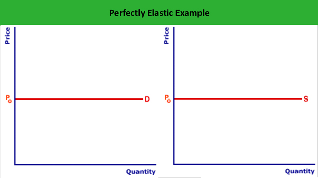
elasticity = infinity
infinitely responsive demand/supply to price
Perfectly inelastic
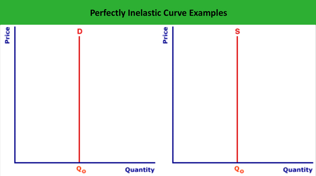
elasticity = 0
demand/supply not responsive to price
Determinants of price elasticity of demand
availability of close substitutes
more substitutes → more elastic
passage of time
more elastic over long time periods
luxuries vs necessities
luxuries = more elastic than necessities
definition of the market
more narrowly defined market → more elastic
willingness to search
more willing to search → more elasticity
Total expenditure
total revenue = P x Q
If demand is price elastic → ∆Q > ∆P → quantity effect dominates
if P increase → TR decrease
If demand is price inelastic → ∆Q < ∆P → price effect dominates
if P increase → TR increase
elasticity on a linear demand curve
linear demand curve
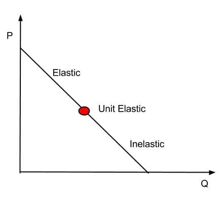
upper half → elastic
lower half → inelastic
middle point → unit elastic
total revenue curve
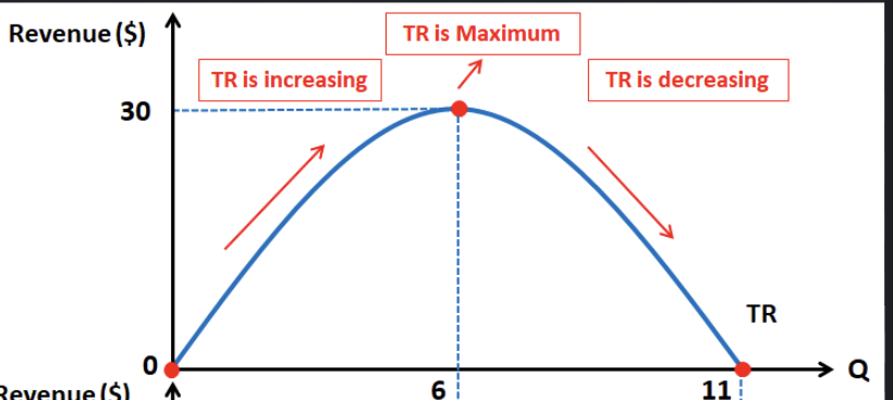
middle → total revenue is maximized
lower quantities
price decrease + TR increase
quantity effect
higher quantities
price decrease + TR decrease
price effect
income elasticity of demand

how quantity demanded responds to changes in income
normal good
> 0 (positive)
luxuries
E > 1
income elastic
necessities
0 < E < 1
income inelastic
inferior goods
< 0 (negative)
cross-price elasticity of demand

how quantity demanded responds to change in the price of another good
substitutes in consumption
E > 0
P of x increases → consume more of y
complements in consumption
E < 0
price of x increases → consume less of y
Determinants of the price elasticity of supply
availability of inputs
increased availability of inputs → elasticity increases
inventories
more stuff firms have → elasticity increases
extra capacity
more excess capacity → higher price elasticity
ease of entry/exit
easier to enter/exit market → higher elasticity
time
supply is more elastic over time
Price ceilings
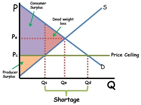
max legal price in a market
ex. rent control
price always below equilibrium
shortage
consequences
shortages
secondary markets (ex. resellers)
consumers who can find/purchase are better off
prices are lower
consumers who cannot purchase good/service are worse off
producers are worse off
lower profits
price floors
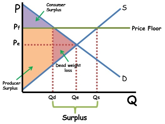
minimum legal price in a market
ex. minimum wages
price always above equilibrium
surplus
Consequences
surplus
producers who can still sell good/service are better off
producers who can no longer sell good/service are worse off
consumers are worse off
quota
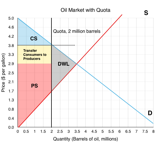
legal max on quantity bought/sold in a market
taxes

per unit taxes - help govt raise revenues to be spent on public goods
put a wedge btwn price buyers pay + price sellers recieve
difference goes to govt
decrease quantity sold in market
buyers pay more
sales tax
Pb = Ps + tax
Pb = demand curve
sellers get less
excise tax
Ps = Pb - tax
Ps = supply curve
implementing taxes on buyers leads to same outcome as putting taxes on sellers
formulas
TR = tax x Qtax
CS = ½ (Pmax - Pb) x Qtax
PS = ½ (Ps - Pmin) x Qtax
DWL = TS0 - TStax
Tax burden
falls on side of market that is more inelastic
Buyers
(Pb - P)/tax
Sellers
(P - Ps)/tax
Subsidies
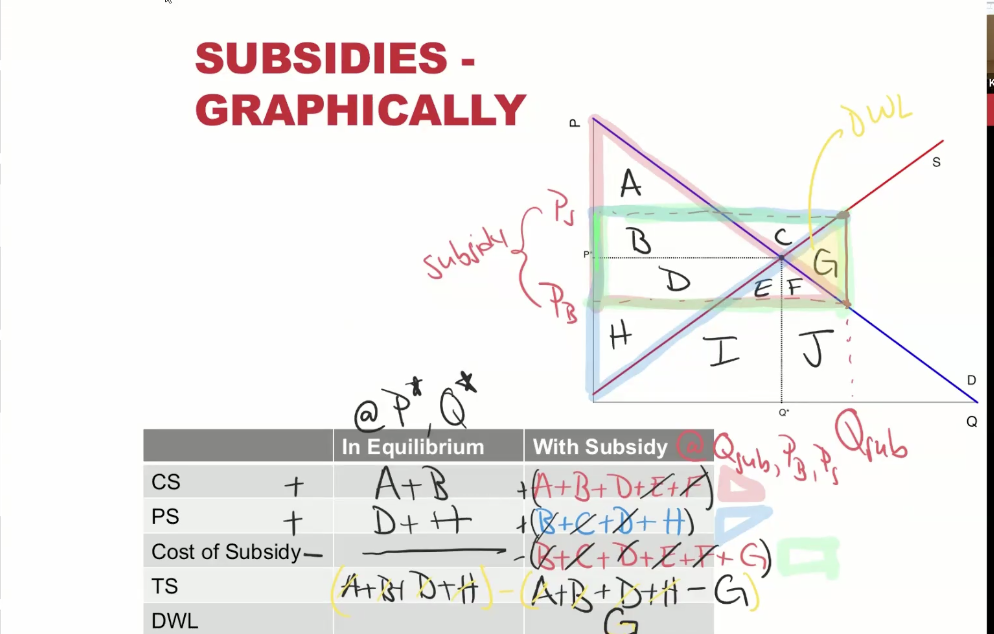
payments made by govt to producer/consumer
effect will be the same no matter who its given to
buyers
Pb = Ps - subsidy
sellers
Ps = Pb + subsidy
increase quantity sold in market
Coase Theorem
private bargaining → efficient outcomes regardless of who holds property rights
applies only in absence of transaction cost
govt solutions to externalities
pigovian taxes/subsidies
tax - MEC
subsidy - MEB
4 categories of goods
excludable - product/service ppl are prevented from using if they don’t pay
non excludable - product/service ppl cannot be stopped from using
rival - consumption of goods prevents others from buying them
private goods (excludable)
ex. candy bar
common resources (non-excludable)
ex. apple trees in quad
non rival - consumption of goods does not prevent others from buying them
artificially scarce goods (excludable)
ex. HBO, netflix
public goods (non-excludable)
ex. roads
public goods
problem
free riding
solution
central protection w mandated payments
common resources
problem
tragedy of commons
aka overuse
solution
assign property rights
make excludable
MIDTERM 2
macroeconomics - study of economy as a whole
Gross Domestic Product (GDP)
market value of all final goods/services produced in a country in a year
not quantities, but what output is worth at market prices
goods are bought for use by final user
NOT INTERMEDIATE GOODS
intermediate goods - goods that are made for something else (ex. ink for a marker)
avoid double counting
measure production
not sales
produced within a country’s borders
ex. an american company produces a car in mexico → value of car counted as part of Mexico’s GDP
used to measure the economy
grey bars on a GDP graph = recessions
Limitations of GDP
excludes non-market activity
parenting, caregiving, home cooking, volunteering, etc
ignores underground/informal/shadow economy
cash jobs, barter systems, illegal transactions, etc
Fails to account for income distribution
Disregards environmental damage
Ways to calculate GDP
Methods
value added approach
add up additional value created in each stage of the production process.
Income method
add up income generated by production
Expenditure method
add up spending on goods/services
Formula
Y = C + I + G + NX
Y = GDP/Output/Income
C = consumption spending
household spending on goods/services
I = investment spending
firms spending on physical capital goods
businesses spending on themselves
factories, buildings, machinery, etc
also changes in inventories
goods produced BUT not sold
G = govt spending
govt purchases of goods/services
paying workers, buying tar for roads, buying trucks for park service, pay interest on debt, tax credits, SNAP benefits, etc
NOT transfer payments
govt writing checks to ppl
NX = net exports
exports - imports (X - M)
add in any money spent by foreigners on things produced in US
subtract anything that consumers, businesses, or govt purchased that produced abroad
GDP per Capita
GDP per person
GDP/population
allows to conceptualize very large number + compare living standards across countries
Gross National Product (GNP)
value of final goods/services produced by americans
not necessarily within US borders
World Happiness Index
alternative measure of well-being
Nominal vs Real GDP
nominal GDP
value of all final goods/services measured in current year prices
Real GDP
value of all final goods/services measured in constant prices
base year specified
chain weighting
calculating real GDP growth btwn 2 years → average prices btwn 2 years
Q of current year x P of base year
Circular Flow Model

2 sides
households
provide inputs to businesses
get paid in income (wages, profits) in exchange
use it to spend on goods/services
buy outputs from businesses
businesses
use inputs from households → outputs
interacting in 2 markets
inputs
labor/physical capital
outputs
goods/services
the rule of 70
amount of time it takes GDP to double is
70/g
g = annual growth rate
answer = years to double
Calculating growth rates

economic growth model
economic growth = increasing real GDP per capita
standard of living
how to increase output
more labor (L)
ex. workers
more physical capital (K)
equipment, factories, buildings, etc
more human capital (H)
knowledge/skills of workers
tech progress
combining inputs to make outputs
Production function

Y = f (L, H, K)
assume constant returns to scale
ex. double inputs → double outputs
output per worker
Y/L = f (K/L, H/L)
Aggregate production function

horizontal axis - physical capital per worker (K/L)
vertical axis - RGDP per worker (Y/L)
aka output per worker
more physical capital per worker → more output per worker
over time, slope gets smaller and smaller
increasing amount of workers using the same amount of capital → oversaturation → production levels off
Movement
change in physical capital per worker (K) → movement along curve
increases get smaller and smaller the more physical capital per worker we already have
diminishing marginal returns
Shifting
change in human capital (skills) (H)
change in technology (T)
due to changes in efficiency
Technological process = key to economic growth
ideas
can be freely shared
nonrival
just bc youre using an idea doesnt mean somebody else cant
do not depreciate w use
don’t wear out
promote other ideas
nonexcludable
why do economies fail to grow?
govt/institutions
Unemployment
Classifying population
Working Age Population (P)
16+ years old
In labor force (LF)
#employed + #unemployed
not in labor force (NLF)
not working/seeking work
Employed (E)
anyone w a job
includes part time
Unemployed (U)
not working BUT seeking work
Definitions
Labor Force Participation Rate
LF/P x 100
employment population ratio
E/P x 100
unemployment rate
U/LF x 100
natural (equilibrium) rate of unemployment
rate of unemployment when economy operating at capacity
frictional + structural
underemployment
people are employed but work part time instead of full time
work less hours than desired
working a job far below education, training, or skill level (overqualified)
still count as employed in U-6
missed in U-3
marginally attached workers
people who want to work and looked for a job in the last year, but are not currently searching
discouraged workers
do not believe jobs are available
not in labor force for U-3
counted in U-6
Types of unemployment
frictional
unemployment due to time spent searching for a good job match
structural
unemployment bc of mismatch btwn skills of workers vs skills needed by employers
OR from wages above equilibrium level
excess supply of labor
OR location (ex outsourcing)
cyclical
unemployment bc of recessions
Inflation
growth in price levels
Inflation rate

hyperinflation
extreme rapid increase in prices
costs of expected inflation
shoe-leather costs
increased costs of transactions caused by inflation
menu costs
real cost of changing listed prices
confuses signals that prices send
do people actually want more stuff?
should producers produce more?
redistribution
actual inflation is higher than expected…
borrowers better off
lenders worse off
actual inflation is lower than expected…
lenders better off
borrowers worse off
Consumer Price Index (CPI)
measures cost of purchasing a market basket of a typical household’s consumption

meanings
100 = base year
> 100 = prices in t > prices in b
< 100 = prices in t < prices in b
challenges
substitution bias
ppl switch away from things that get pricier
quality bias
higher price might mean a better product
new product bias
new, cheaper options aren’t in basket yet
leads to CPI slightly overstating inflation consumers face
Personal Consumption Expenditure Deflator (PCE deflator)
used by federal reserve
similar to CPI w continuously updated basket
GDP deflator

a measure of price level of things produced in the economy
GDP deflator in base year = 100
nominal = real
meaning
100 = base year
> 100 = prices in t > prices in b
< 100 = prices in t < prices in b
producer price index (PPI)
measures prices producers face
can be early warning of increase in consumer prices
real vs nominal variables
nominal
measured in that years dollars
real
adjusted for changes in price level
measures purchasing power in base year dollars
real wage
nominal wage/price index x 100
what your paycheck can actually buy
real income
nominal income/price index x 100
Same idea, for all earnings
real interest rate
nominal rate - inflation rate
what your savings really earn
interest rate = return to savings & cost of borrowing
money vs wealth vs income
money
assets people use to buy things
cash/checking deposits
wealth
everything you own - everything you owe
measured at a point in time
income
earnings over a period of time
history of money
barter economies
trade goods/services directly for other goods/services
needs double coincidence of wants
2 parties each have an item the other person wants
trade w commodity money
has intrinsic value
ex. gold/silver
trade w paper money
IOU
backed by a commodity
trade w fiat money
no intrinsic value
valuable bc ppl think its valuable
Functions of money
medium of exchange
smth sellers are willing to accept in exchange for goods/services
unit of account
way to measure value
each good has a single price
store of value
money has to stay valuable over time
Banks
main function
pool savings from many savers
collects deposits form savers → use funds to support lending
spread risk of lending across many borrowers
lend to many borrowers instead of concentrated risk on one loan
solve info problems
evaluate borrowers + monitor loans → reduce risks w lending
provide payment services
facilitate transactions via checking accounts, transfers, etc
create long term loans from short term deposits
use deposits → fund loans repaid over many years
fractional reserve banks
banks have to keep some fraction of deposits on reserve at all times
can loan out rest
in depth explanation
Depositors can ask for a certain amount
ex. 1k
the bank has a fraction of it in the vault
ex. 100
the other part is involved in car loans, mortgages, business loans, etc that pay back over years
ex. 900
Owns
fraction in reserves (in the vault)
100
fraction in loans
900
Owes
deposits
1000
banks cannot pay back all depositors at once if everybody comes to claim their money
bank runs
a bunch of people try to withdraw money all at once
FDIC provides deposit insurance
makes sure that money in deposit acc is protected for the depositor
What if banks don’t have enough in reserves?
borrow from other banks → pay FFR
borrow from Fed → pay discount rate
discount rate = ceiling on FFR
DR has to be higher than FFR for banks to borrow from each other
What if banks have excess reserves?
loan to other banks → earn FFR
earn interest on reserves held by FED
only some institutions
loan to FED in an overnight reverse repurchase agreement
earn ON RRP rate
price floor on FFR
Stocks and bonds
Bond
IOU
company/govt issue bonds to borrow money
promise to pay back w interest
treasury bonds
issued by govt when it spends more than brings in on revenue
You buy bonds → you get paid interest
You issue bonds → you pay interest
Stock
partial ownership of a firm
have a say in how company is run
get paid dividends
company is more valuable when they sell stock → can make money
Business cycle
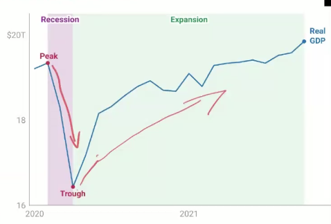
short run fluctuations in economic activity
stages
peak
high point of econ activity
trough
low point of econ activity
recession
declining econ activity
peak → trough
expansion
increasing econ activity
torugh → peak
continues until adverse shock
potential output
level of output occurring when resources fully employed
what we can sustainabley produce given current resources/technology
long run economic growth → growth in country’s potential output
the output gap

difference btwn actual and potential output
actual - potential
measured as percentage of potential output
meaning
< 0 = economy producing less than potential
> 0 = economy producing more than potential
Leading Indicators
variables that tend to predict future path of economy
gives sense of where economy is headed
tend to change first
examples
business confidence
consumer confidence
stock market
Lagging Indicators
variables that tend to follow business cycle movements w delay
examples
unemployment
inflation
Indicators
Real GDP
broadest measure of economic activity
measures total size of economy
incomplete when first released
Real GDI
cross check on GDP
adds up total income
more reliable than GDP
Nonfarm Payrolls
tell if labor market is improving
how many jobs are created each month
tracks number of workers on business payrolls
Unemployment rate
indicator of excess capacity
share of labor force that wants a job but can’t find one
Initial unemployment claims
timely indicator
how many people lost jobs + applied for unemployment insurance during previous week
business confidence
what managers are planning
Supply Management’s Purchasing Manager’s Index
Consumer Confidence
what consumers are thinking
asks regular people how optimistic they are about the economy
Iinflation rate
whats happening with prices
CPI → how much economy wide prices are growing
employment cost index
whats happening with wages
how fast wages/benefits are rising
leading indicator of inflationary pressure
stock market
future expected profits of business
“predicted 9 out of the last 5 recessions”
Aggregate Demand
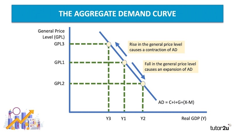
curve that shows relationship btwn price level and total quantity of output buyers collectively plan to purchase
buyers = consumers, businesses, govt, foreigners
movement
changes in price level
Wealth effect
price increase → savings worth less → C decreases
Fed Channel
price increase → Fed raises real IR → cost of borrowing increases + return to savings increases → I and C decrease
International Trade effect
price increase → US goods look pricier → NX decrease
Shifts
change in spending
increase → AD shifts right
decrease → AD shifts left
Shifters of AD
Consumption: What makes households spend more?
Wealth
wealth increases → C increases
Consumer confidence/expectations
expect higher prices in future → current C increases
Taxes + govt assistance
can only spend disposable income (Yd)
Yd = Y - taxes + transfers
transfers = tax credits, income assistance, housing subsidies, etc
taxes decrease OR transfers increase → consumption increases
Redistribution to people more likely to spend
marginal propensity to consume (MPC)
fraction of one’s disposable income that is spent
lower incomes → higher MPC
higher proportion of money spent on necessities → lower proportion of money that can be saved
Investment: What makes businesses spend on physical capital?
an expanding economy
more people want to buy goods/services → businesses will spend more to supply
business confidence
higher confidence → more confidence making physical investments
lower corporate taxes
low taxes → higher returns on physical capital investments
lending standards + cash reserves
more cash on hand → easier to make investments
easier/cheaper to borrow money → more investment spending
aka lower IR
less uncertainty
less uncertainty → more likely to spend on capital
govt purchases: What changes how much the govt spends?
politics
spending bills
war
Net Exports: What changes how much foreigners want to purchase from us and how much we want to purchase from foreigners?
global economic growth
foreigners become wealthier → they have higher incomes → want to buy more stuff → buy more American stuff
exchange rate
USD appreciates (costs more foreign currency to buy 1 dollar)
US stuff becomes more expensive for foreigners → exports decrease
foreign stuff now cheaper for americans → imports increase
NX decrease
USD depreciates (costs less foreign currency to buy 1 dollar)
US stuff becomes cheaper for foreigners → exports increase
foreign stuff now more expensive for americans → imports decrease
NX increase
Trade barriers
import quotas/tarriffs
trade war → impose tariffs on a country → restrict their imports
country imposes tariffs on use → restrict our imports
net effect depends on whos imposing more/higher tariffs
Short Run Aggregate Supply

relationship btwn aggregate price level and quantity of output producers are willing to supply
output rises → excess demand → prices rise
output falls → insufficient demand → prices fall
Shifters of SRAS
changes in input prices (including wages)
higher price of inputs → more expensive to produce → firms have to charge higher prices → shift SRAS left
lower price of inputs → less expensive to produce → firms charge lower prices → shift SRAS right
higher import prices
lots of inputs are imported
import prices are higher → input prices increases → SRAS shifts left
depreciating USD
raises production costs
for imported intermediate goods
more expensive
increases competitiveness of US goods → firms charge higher prices for same level of output
Long Run Aggregate Supply

real level of GDP producers are willing to supply is determined by
supply of labor
supply of capital
physical + human
technology
NOT PRICE LEVEL
in long run, all prices (including wages) move together
intersection of AD, SRAS, and LRAS → LR macroeconomic equilibrium
we are producing at potential output
intersection of AD and SRAS → SR macroeconomic equilibrium
not at potential output
Shifts in SRAS and LRAS
LRAS cannot shift without shifting SRAS
changes in productivity
technological change
changes in human capital
increase in tech or human capital → LRAS + SRAS shift right
changes in labor force + capital stock
increase in L or K → LRAS + SRAS shift right
Macroeconomic equilibrium

Long Run: Y = Yp
Short run: AD = SRAS
all 3 cross at one point → economy is in short and long run equilibrium
Adjustment from SR → LR
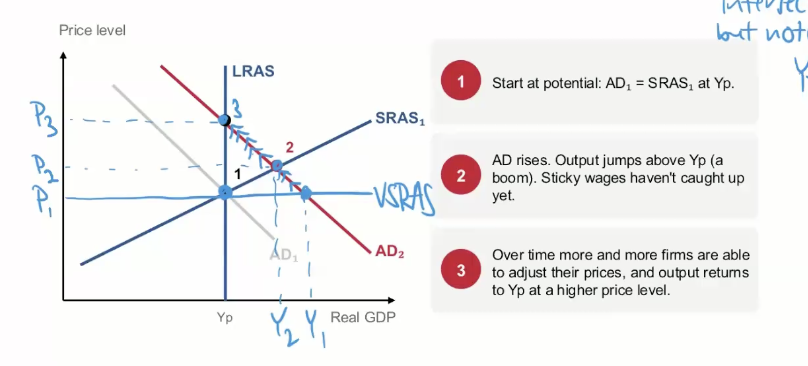
sticky prices
prices that adjust sporadically/sluggishly to changes in market conditions
aka it takes time for prices to adjust
in very short run → prices are completely sticky/cannot change → only output can adjust
in short run → firms see output is higher than potential output → excess demand for output → prices push up
not all firms do it at the same time → SRAS changes
more firms adjust prices → get to new LR equilibrium → back at potential output
all prices fully adjusted
basically: change in AD → push prices, but since nothing changed potential output → pushes RGDP in short run → prices adjust back in long run → back at potential output
Shocks
unexpected events that shift AD or SRAS curves → move economy away from long run equilibrium
positive → right
negative → left
Monetary Policy
central bank’s control of money supply + IR to achieve macro policy goals
Who: The Federal Reserve (FED)
created in 1913
board of governers in DC + 12 district banks
independent
governers appointed by president + confirmed by senate
Why: Dual mandate
maintain price stability
2% inflation target
promoting max sustainable employment
How: Interest Rates
steers short term investment rates
IR change spending → shift AD
*consumers like low IR
Tools to set a target inflation rate (2%)
set IR paid on reserves
rate for FED borrowing from banks
banks can leave excess reserves at FED → like loaning money to the FED → get paid interest
increase IR → banks get higher return for keeping money at FED → banks charge consumers higher IR for loans → C + I decrease
decrease IR → banks earn less for keeping money at FED → incentivized to lend it out → banks charge consumers lower IR for loans → C + I increases
set rate of return for overnight reverse repurchase agreements
rate for FED borrowing from banks
directly loan money to FED
increase ROR → private borrowers have to match/exceed rate to attract cash → borrowing costs increase → C + I decrease
ROR = IR that fed pays
set discount rate
rate at which banks borrow from FED
increase DR → more expensive to borrow → I + C decrease
open market operations
buying/selling of govt bonds on open market
FED buys bonds → bank is paid and gets more reserves → IR decreases → C + I increase
used to be main monetary policy tool
Federal Open Market Committee (FOMC)
meets 8 times a year → announces new IR target
Look at
inflation rates
output gaps
Steering fed funds rate
Fed has 2% inflation target → targets FFR to achieve it
Taylor Rule
“Fed rule of thumb”
FFR - inflation = neutral real rate + 0.5 ( inflation -2%) + output gap
FFR = nominal short term interest rate
Recommended FFR is above today’s FFR → raise
Recommended FFR is below today’s FFR → cut
neutral real rate
interest rate that supports max sustainable employment
0.5 ( inflation -2%)
how far inflation is from 2% target
inflation father away → raise rates
output gap
output (Y) > potential output (Yp) → raise rates
Why do we care about IR?
FFR rises → other IR rise
borrowing cost increases
saving pays more
Fed raises target FFR → mortgage, car loan, savings rates rise → spending changes
households
saving vs spending
return to savings increases → spend less (C decreases) → AD decrease
firms
borrowing to invest
cost of borrowing increases → investment decreases → AD decrease
The rest of the world
the value of the dollar
USD appreciates → increase imports + decrease exports → NX decreases → AD decrease
All 3 → AD shifts left
Expansionary vs Contractionary monetary policy
expansionary
used for negative output gaps (Yo < Yp)
IR falls
AD shifts right → economy pushed up to LR equilibrium
contractionary
used for positive output gaps (Yo > Yp)
IR rises
AD shifts left → economy pushed down to LR equilibrium
Fiscal Policy
changes in govt spending, taxes, or transfers in order to achieve macroeconomic policy objectives
people (C) will spend some amount regardless of disposable income (a)
but some parts dependent on income (MPC)
C = a + MPC (Yd)
a = autonomous consumption spending (not dependent)
MPC = marginal propensity to consume
fraction of disposable income that gets spent
Yd = disposable income
Yd = Y - taxes + transfers
who: elected officials via budget/tax laws
Tools
govt purchases (G)
taxes
taxes increase → less disposable income → AD decreases
taxes decrease → more disposable income → AD increases
transfer payments
transfers decrease → less disposable income → AD decreases
transfers increase → more disposable income → AD increases
Expansionary vs Contractionary fiscal policy
expansionary
increase govt spending
decrease net taxes
decrease taxes
increase transfer payments
AD shifts right
contractionary
decrease govt spending
increase net taxes
increase taxes
decrease transfer payments
AD shifts left
govt purchases mulltiplier

increase in govt purchases → increase income → increase consumption → increases income → increase consumption → etc.
basically… initial increase → larger change in output
multiplier effects of taxes and transfers

decrease in taxes OR increase in transfers → increase income → increase consumption → increase income → increase consumption → etc.
lower than govt purchases multiplier
changes in taxes/transfers → don’t change all spending initially
part of the change is saved
negative bc lowering taxes raises GDP + raising taxes lowers GDP
Automatic stabiliziers
govt spending/taxes that automatically adjust with business cycle
timely, targeted, temporary
ex. income taxes, unemployment insurance
Discretionary fiscal policies
govt takes action to change taxes, transfers, and purchases to affect business cycle
ex. stimulus checks, income tax cuts
issues w fiscal policy
legislative lags
need many different opinions to agree → takes time for decisions to come out
shocks can already pass before decision is made
crowding out of private investment
govt spends money (expansionary) → need to borrow money → pushes IR up for other borrowers → crowd out private investment
increase G → decrease I
Types of Taxes
progressive
ppl w higher incomes → pay higher fraction of income in taxes
income rises → avg tax rate rises
ex. US income tax system
proportional
ppl pay same fraction of income in taxes regardless of income
avg tax rates independent of income
ex. flat tax
regressive
ppl w higher incomes → pay lower fraction of income in taxes
income rises → avg tax rate decreases
ex. sales + excise taxes, payroll taxes, property taxes
fiscal policy and federal budget
budget balance = tax revenues - govt purchases - transfers
> 0 = budget surplus
< 0 = budget deficit
0 = balanced budget
budget deficit → govt adds to national debt via borrowing
budget surplus → pays the debt
national debt = sum of past deficits - sum of past surpluses
Should we worry about the debt
reasons not to worry
US debt = money owed by americans to americans
future generations can help repay debt
not a big adjustment to repay
govt doesnt need to fully repay debt for it to be sustainable
govt has options you dont
taxation, printing money, etc
reasons to worry
slower economic growth
future spending might be constrained
risk of debt crisis rises
risk of not being able to actually pay
crisis of confidence
ppl think you might not be able to pay debt → charge higher interest
import or export
autarky (AUT) = no trade
world market made up of global consumers of good
world market determines world price
domestic market made up of domestic consumers of good

Pw < Paut → import
consumers better off
producers worse off
domestic price falls to Pw
gap = imports
Pw > Paut → export
producers better off
consumers worse off
domestic price rises to Pw
gap = exports
Pw = world price
Paut = autarky price
Pw and Paut prices compete
choose btwn whichever is cheaper

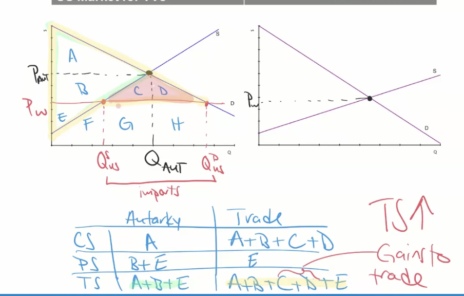
either way, free trade increases total surplus
winners gain more than losers lose
Why restrict trade?
concentrated gains, spread out losses
few producers lose a lot
millions of consumers each gain a little
jobs/adjustment
workers in import-competing industries bear the costs
national security
keep ability to produce key goods at home
revenue and bargaining
tariffs raise money → can be used as leverage
Policies restricting trade: tariffs
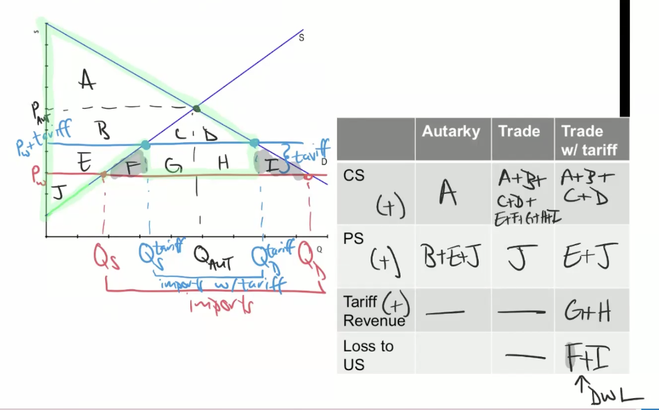
alters price → influence imports
import tariff imposed when Pw < Paut
push price of good in US up by tariff
Pw + tariff
# imports fall
Policies restricting trade: import quotas
same impact on producer/consumers as a tariff
places limit on how much can be imported → influences price
quota rents - extra profit created form imports
goes to foreign producers

Foreign exchange markets
market where currency of one country traded for currency of another
exchange rate = price of one USD in terms of other currency
Law of demand and supply in foreign exchange markets
ppl demand USD → buy US produced goods/services + assets
ER increases → price of USD increases → Qd of USD decreases
ppl sell USD → buy foreign produced goods/services + assets
ER increases → what you can get in exchange increases → Qs of USD increases
exchange rate based on supply/demand for USD in foreign exchange market
Equilibrium in Foreign Exchange Markets

demand from ppl holding foreign currency
supply from ppl holding domestic currency
switch graph labels based on currency exchanged
Y axis equilibrium (foreign currency/domestic currency) labeled as E
represents nominal exchange rate
ER increase for country X → X appreciates → Y depreciates
ER decrease for country X → X depreciates → Y appreciates
One market, two currencies
europeans want US goods/services + assets → sell euro + buy USD → demand for dollar = supply of euro
Americans want european goods/services + assets → sell USD + buy euro → supply for dollar = demand of euro
USD appreciates → Euro depreciates
Euro appreciates → USD depreciates
shifts of demand for USD in foreign exchange markets
value of US exports
strength of global economy
barriers to trade in foreign markets
domestic innovation + marketing
foreign prices
domestic prices
financial inflows into US
interest rate differentials
business profitability
political risk
changes in expected exchange rate
shifts of supply of USD in foreign exchange markets
value of imports into US
strength of domestic economy
trade barriers protecting domestic producers
foreign innovations + marketing
domestic prices
foreign prices
financial outflows from the US
interest rate differentials
business profitability
political risk
changes in expected exchange rate
A strong dollar: who wins?
winners
US tourists broad
US buyers of imports
US firms buying foreign assets
Losers
US exporters
US tourism businesses
US firms earning abroad
purchasing power parity
in longrun → ER should move to equalizing purchasing power across different currencies
ex. if a burger costs $2 in the US + ER is 0.76 euros/USD → the same burger should cost $2 × 0.76 euros/USD = 1.52 euros
real vs nominal exchange rates
foreign exchange markets = nominal exchange rate
real exchange rate shows how prices of goods/services compare in 2 countries
for one item

overall

real exchange rates + trade
real ER
determine competitiveness of US firms broadly
high RER → american prices high relative to foreign prices
low RER → american prices low relative to foreign prices
drives imports/exports
RER increases → american goods more expensive for foreigners + foreign goods cheaper → NX decreases
RER decreases → american goods cheaper for foreigners + foreign goods moere expensive → NX increases
different exchange rate policies
floating
ER determined by supply/demand in foreign exchange markets
US dollar, euro, yen, pound
fixed (pegged)
ER fixed to another currency
ex. danish krone is tied to euro at 7.46 kr/euro
managed
govt buys/sells currency in foreign exchange markets → reduce volatility and/or keep currency/exports cheap
ex. chinese yuan; central bank sets daily reference rate where trading allowed within +- 2% of it
FINAL
Production function

tells max amt of output a firm can produce using different combinations of 2 inputs
labor (L)
workers, hours
capital (K)
physical capital (machines, buildings, ovens)
Long run vs Short run
short run (SR)

at least one input is fixed (capital)
we cannot change the capital we already have
labor is variable
long run (LR)

all inputs are variable
new tech, bigger plant, or exit
SR and LR have different lengths for different firms
depends on how long it takes to change capital
ex. short run for a company w a 5 year lease on an office space is longer than short run for a company with a 1 year lease
production in short run
total product (quantity or output)

amount produced in a given time period
average product of labor

total product divided by total number of workers used in production
marginal product of labor

additional output produced due to hiring an additional worker
TP, MPL, and APL on a graph
Y axis = quantity
X axis = labor (L)
MPL = slope of TP
TP
upwards sloping
initially slope is increasing
range of output where adding workers to fixed input can increase productivity
adding additional units of variable input → diminishing marginal returns
adding variable input (labor) to fixed input (capital) → eventually lowers MPL
MPL
increases then decreases after some point
marginal pulls average
MPL > APL → rising APL
MPL < APL → falling APL
MPL and APL intersect at APL’s maximum
APL
Costs
explicit costs
costs that involve spending money
ex. rent, wages, materials, utilities
implicit costs
nonmonetary opportunity cost
ex. forgone wages, forgone interest on your own money
accounts count explicit costs, economists count both
costs in the short run
total cost (TC)

cost of all inputs a firm uses in production
total fixed cost (TFC)
cost that remains constant as output changes
total variable cost (TVC)
cost that changes as output changes
average/marginal costs in the short run
average total cost


average variable cost
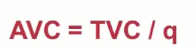
average fixed cost

falls as q rises
marginal cost

change in total cost from 1 unit change in output
Cost curves

MC is U shaped
mirror of MPL
AFC falls forever
ATC - AVC = AFC → gap shrinks
MC crosses AVC and ATC at minimums
marginal pulls the average
MC < ATC → ATC + AVC are falling
MC > ATC → ATC + AVC are rising
MC = ATC → ATC at minimum
MC crosses it here
Revenue
amount of money a business/govt gets from activities before expenses are subtracted
Total revenue

average revenue

marginal revenue

Profit

total revenue - total cost

P - ATC = profit margin
profit per unit
q = number of units
Accounting profit
total revenue - explicit costs
economic profit
total revenue - explicit costs - implicit costs
economic profit ≤ accounting profit

4 market structures
no market power → full market power
perfect competition
many firms
identical products
no barriers
key trait = price taker
no individual firm’s actions affect market price
ex. wehat, corn
mopolistic competition
many firms
differentiated product
no/few barriers
key trait = some control over price
ex. restaurants, coffee shops
oligopoly
few firms
identical or differentiated products
significant barriers
key trait = strategic/watches rivals
ex. cell service, airlines
monopoly
one firm
unique, no close substitute products
very high barrier
key trait: price maker
has full control over how price is set in industry
ex. local water utility
Where does market power come from?
poduction differentiation
product is different → customers don’t all leave when price raises
products become imperfect subtitutues
lack of competition
barriers to entry → keep rivals out → buyers have fewer places to go
market power
ability to raise prices without losing all customers
Firm demand curves (INSERT PICTURE)
more market power → steeper demand curve
demand curve a firm faces depends on how easily it buyers can switch to a rival
perfect competition
market decides P*
each firm is a price taker
can sell as much as it wants at P*
Revenue
AVG revenue = P*
Marg revenye = P*
for a price taker every extra unit sells for P → each adds exactly P to revenue
firm’s demand curve = MR curve
profit maximization = firm’s goal
Profit = TR - TC
q increases
TR increases → MR tells us how much
TC increases → MC tells us how much
rational rule for sellers
sell one more unit if MR ≥ MC
firms produce where MR = MC
firms’ profit max condition
MR > MC → increase Q → increase profits
MR < MC → decrease Q → increase profits
firms set price from demand curve
in PC markets → P = P*
Per unit vs Total Profit
Profit = TR - TC
profit = (P x q) - (ATC x q) = q x (P - ATC)
P - ATC = per unit profit
P = ATC → firm is breaking even
economic profits = 0
accounting profit ≥ 0, but firm is doing just as well as they could be in next best option
perfectly competitive firms → break even occurs where
P* = MR = MC = minATC
Three steps: output, price, profit
Find q* where MR = MC
Find p*: read up to demand curve at q*
price taker: p* is given
find profit: profit = q* x (p* - ATC at q*)
The short-run shutdown decision
short run → fixed costs are sunk
Operate (q > 0)
profit = TR - VC - FC
Shut down (q = 0)
profit = -FC
TR > VC → operate
ie. P > AVC
P < AVC → shut down
The firm’s short run supply curve
at any price → firms pick q where P = MC
as long as P ≥ min AVC
market supply adds up all firms
100 identical firms → 100 x q at each price
rational rules for entry/exit in the long run
expectation of positive economic profit → enter
expectation of negative economic profit → exit
w free entry and exit → market supply shifts until economic profit = 0
in LR, firms dont have an incentive to enter OR exit