Bayes' Nets

Representation

Probabilistic Models

• models describe how the world works

• models are always simplifications

  • may not account for every variable or for all interactions between variables

• need to reason about unknown variables, given evidence

• examples: explanation, prediction, value of information

Independence

• Two variables are independent if:

  • ∀x, y : P(x, y) = P(x)P(y)

    • ∀x, y : P(x | y) = P(x)

    • X ⊥ Y

• Empirical joint distributions: at best “close” to independent

• Ex. N fair, independent coin flips

• Conditional Independence

  • P(Toothache, Cavity, Catch)

    • if I have a cavity, the prob that the probe catches in it doesn’t depend on whether I have a toothache

    • P(+catch | +toothache, +cavity) = P(+catch | +cavity)

    • P(+catch | +toothache, -cavity) = P(+catch | -cavity)

    • Catch is conditionally independent of toothache given cavity:

  • Our most basic knowledge about uncertain environments

  • X is conditionally independent of Y given Z iff:

    • ∀x, y, z : P(x, y | z) = P(x | z) P(y | z)

Bayes’ Nets

• Two problems with using full joint distribution tables as our probabilistic models

• A technique for describing complex joint distributions using simple, local distributions

  • more properly called graphical models

Graphical Model Notation

• nodes: variable (with domains)

  • can be assigned or unassigned

• arcs: interactions

  • similar to CSP constraints

  • indicate direct influence between variables

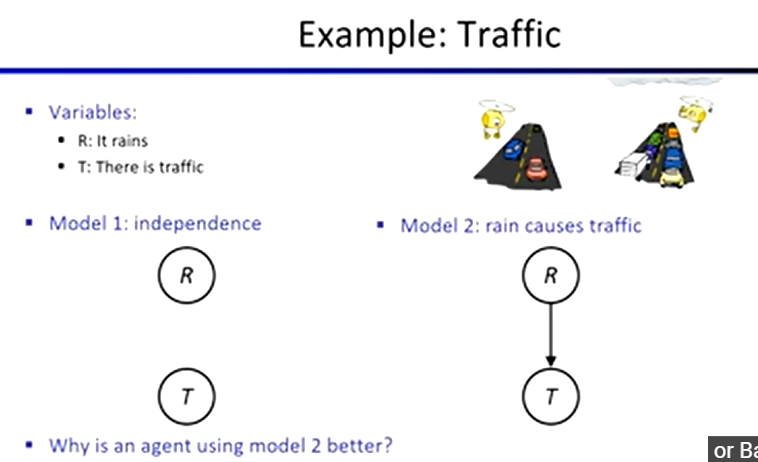
BN Semantics:

• a set of nodes, one per variable X

• a directed, acyclic graph

• a conditional distribution for each node

  • a collection of distributions over X, one for each combination of parents’ values

  • conditional probability table (CPT)

• Bayes Net = Topology (graph) + Local Conditional Probabilities

Probabilities in a BN

• implicitly encode joint distribution

  • as a product of local conditional distributions

  • multiply all relevant conditional together to get probability to a full assignment

• Ex. Coin Flips

  • P(h, h, t, h) = (0.5)⁴

Independence

Size of BN:

• How big is a joint distribution over N Boolean variables?

  • 2^N

• How big is an N-node net if nodes have up to k parents?

  • O(N * 2^k+1)

Assumptions:

• P(x_i | x₁ - - - x_i-1) = P(x_i | parents(X_i))

• conditional independence:

  • W ⊥ X | Y

Casual Chains

• P(x, y, z) = P(x) P(y | x) P(z | y)

Common Cause

• P(x, y, z) = P(y) P(x | y) P(z | y)

Common Effect

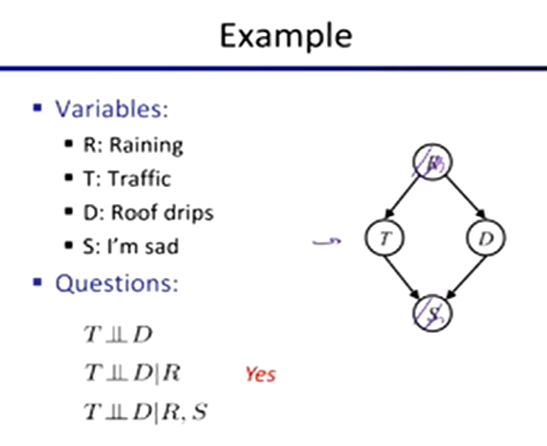
• two causes of one effect (v-structures)

• ex. rain and ball game both would cause traffic

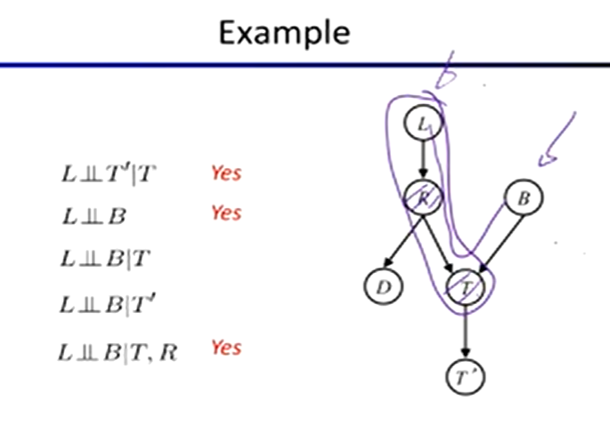
General Question: in a given BN, are two variables independent?

• Solution: analyze the graph

Reachability

• shade evidence nodes, look for paths in the resulting graph

• if two nodes are connected by an undirected path not blocked by a shade node, they are conditionally independent

Active/Inactive Paths

• a path is active if each triple is active

D-Separation

• Query: X_i ⊥ X_j | {X_k1, …, X_kn}

  • check all undirected paths between X_i and X_j

    • if one or more is active, then independence is not guaranteed

    • otherwise (all inactive) independence is guaranteed

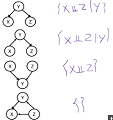
Topology Limits Distributions

• given some graph topology G, only certain joint distributions can be encoded

• the graph structure guarantees certain independences

• adding arcs increases the set of distributions, but has several costs

• full conditioning can encode any distribution

Inference

Probabilistic Inference

• Inference: calculating some useful quantity from a joint probability distribution

  • ex. posterior probability or most likely explanation

Factor Zoo

• joint distribution: P(X, Y)

  • entries P(x, y) for all x, y

  • sums to 1

• Selected joint: P(x, Y)

  • a slice of the distribution

  • entries P(x, y) for fixed x, all y

  • sums to P(x)

• Number of capitals = dimensionality of the table

• Single conditional: P(Y | x)

  • entries P(y | x) for fixed x

  • sums to 1

• Family of conditionals P(Y | X)

  • multiple conditionals

  • entries P(y | x) for all x, y

  • sums to |X|

• specified family P(y | X)

  • entries P(y | x) for fixed y but for all x

  • sums to … who knows!

• In general…

  • P(Y₁ … Y_N | X₁ … X_M)

    • is a “factor”, a multi dimensional array

    • has values of P(y₁ … y_N | x₁ … x_M)

    • any assigned (lower case) X or Y is a dimension missing (selected) from the array

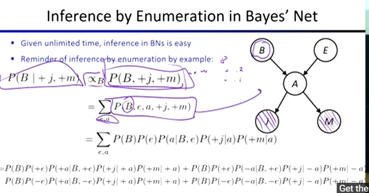
Inference by Enumeration: Procedural Outline:

• track objects called factors

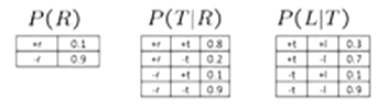
• initial factors are local CPTs (one per node)

• any known values are selected

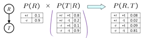
• join all factors

  • just like a database join

  • get all factors over the joining variable

  • build a new factor over the union of the variables involved

    • ex. Join on R

• eliminate all hidden variables

  • marginalization

    • marginalizing early: variable elimination

      • ex.

        

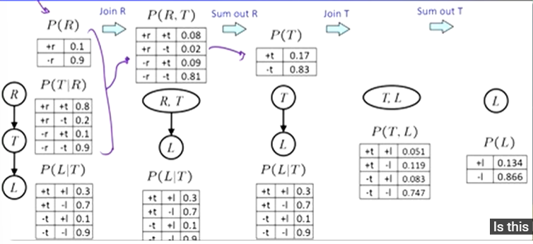
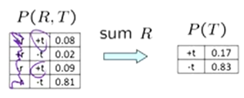
  • take a factor and sum out a variable

    • shrinks a factor to a smaller one

    • a projection operation

  • ex.

    

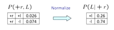
• normalize

Evidence

• if evidence, start with factors that select evidence

  • no evidence uses initial factors

    

  • computing P(L | + r) the initial factor becomes

    

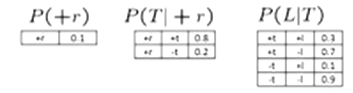
• result will be a selected joint of query and evidence

  

General variable elimination

• Start with initial factors

• while there are still hidden variables (not Q or evidence):

  • pick a hidden variable H

  • join all factors mentioning H

  • eliminate H

• join all remaining factors and normalize

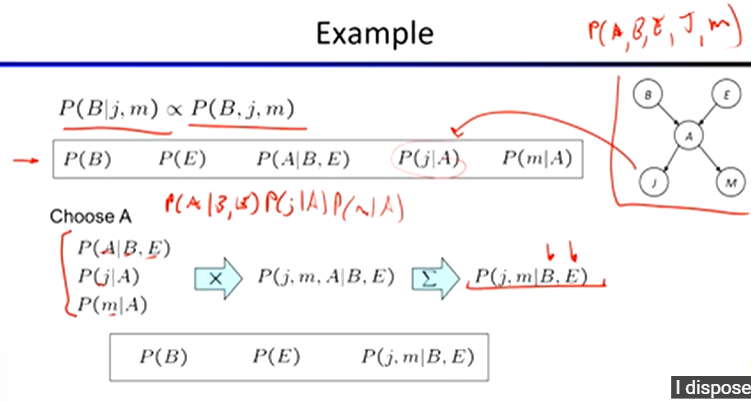
Continued…

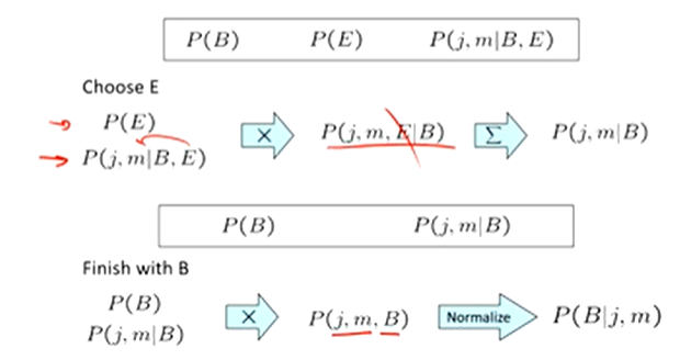
Polytrees:

• a directed graph with no undirected cycles

• can always find an ordering that is efficient

• cut-set conditioning for Bayes’ net inference

Sampling

Approximate Inference: Sampling

• very similar to repeated simulation

• basic idea

  • draw N samples from a sampling distribution S

  • compute an approximate posterior prob

  • show this converges to the true probability P

• Getting a sample is faster than computing the right answer

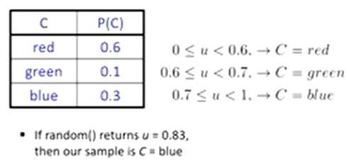
Sampling from a given distribution:

• Step 1: get sample u from uniform distribution over [0, 1)

• Step 2: convert this sample u into an outcome for the given distribution by having each target outcome associated with a sub-interval of [0, 1) with sub-interval size equal to prob of the outcome

• Ex.

  

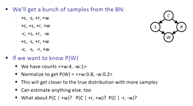
Prior Sampling:

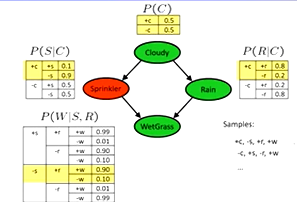
• for i = 1, 2, …, n

  • sample x_i from P(X_i | Parents(X_i))

• return (x_1, x_2, …_, x_n)

• this process generates samples with probability:

  • S_ps(x₁…x_n) = ∏ P(x_i | Parents(X_i)) = P(x₁…x_n)

• let the number of samples of an event be: N_ps(x₁…x_n)

  • lim(N→inf) P(x₁…x_n) = lim(N→inf) N_ps(x₁…x_n) / N = S_ps(x₁…x_n) = P(x₁…x_n)

• the sampling procedure is consistent if the ratio of the samples in the limit goes towards the actual distribution

Example:

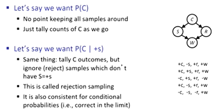
Rejection Sampling

Likelihood Weighting:

• problem with rejection sampling

  • if evidence is unlikely, rejects lots of samples

  • evidence not exploited as you sample

• solution:

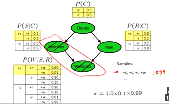
  • fix evidence variables and sample the rest

    • weight by probability of evidence given parents

• Ex.

  

Algorithm:

• input: evidence instantiation

• w = 1, 0

• for i = 1, 2, .., n

  • if X_i if an evidence variable

    • X_i = observation x_i for X_i

    • Set w = w * P[x_i | Parents(X_i)]

  • else

    • Sample x_i from P[X_i | Parents(X_i)]

• return (x₁, x₂, …, x_n), w

Likelihood Weighting:

• Sampling Distribution if z samples and e fixed evidence:

  • S_ws(z, e) = ∏ P(z_i | Parents(Z_i))

• now samples have weights:

  • w(z, e) = ∏ P(e_i | Parents(E_i))

• Together:

  • S_ws(z, e) ⋅ w(z, e) = ∏ P(z_i | Parents(Z_i)) ∏ P(e_i | Parents(E_i)) = P(z, e)

Gibbs Sampling

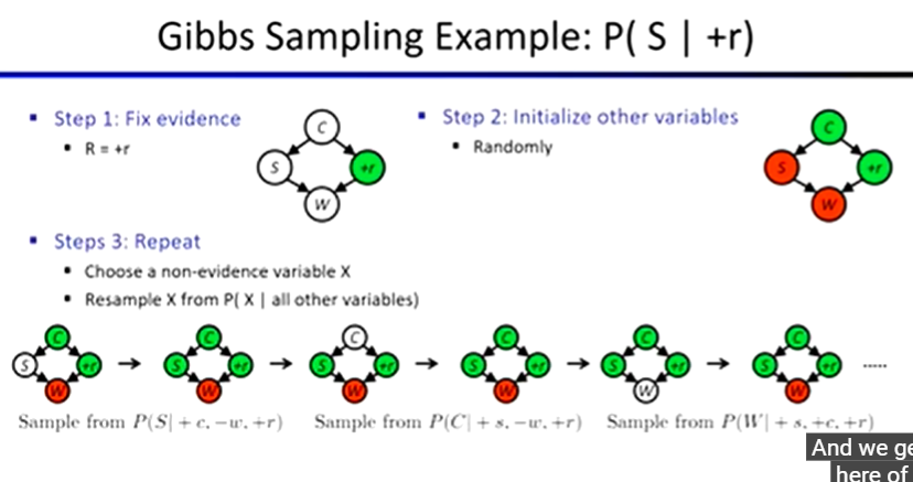
• Procedure:

  • keep track of full instantiation x₁, x₂, …, x_n

  • start with an arbitrary instantiation constant with the evidence

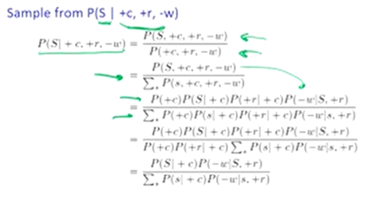
  • sample one variable at a time, conditioned on all the rest, but keep evidence fixed

  • repeat

• Property:

  • in the limit of repeating this infinitely many times the resulting samples come from the correct distribution

• Rationale:

  • both upstream and downstream variables condition on evidence

• Ex.

  

Efficient Resampling of One Variable: