Z-Scores and Standardization (Week 5)
Prior key concepts/lessons that are needed to understand z-scores.
Normal Distributions and how Standard Deviation plays a key role in a normal distribution (first introduced in week 4).
other concepts that tie in…
.. distributions (week 2, mainly refer back to day 2)
Scales of measurement (week 1)
Measures of central tendency (week 3)
Review (week 4)
Standard Deviation:
Standard deviation (SD) is a measure of how spread out the data is.
When a score is many standard deviations away from the mean (like really high or really low), it’s considered “extreme.”
Extreme values are unlikely to occur just by chance if the data follows a normal distribution.
Because they’re rare, we often treat them as “significant” — meaning the value might reveal something important or unique about the situation.
Standard Deviation is used in Normal Distributions.
A Normal Distribution gives us the probability of how likely or rare a score is, and the standard deviation tells us how far that score is from the mean. Together, they let us decide when a value is “extreme” or potentially “significant.”
Normal distributions allow us to get into probability/inference.
We can tell if something is unlikely to happen through the location in the distribution
If and when we find ourselves with a significant score, we can raise the question of “is there something that explains its happening?”
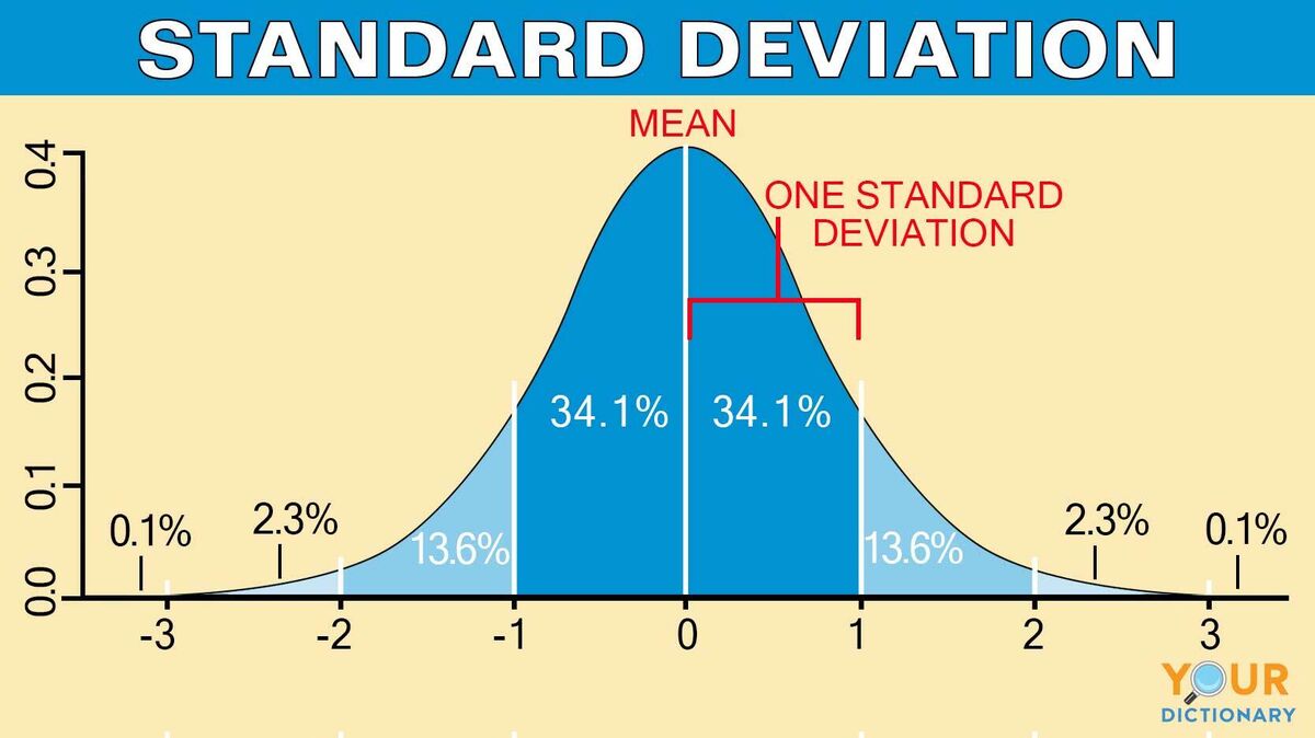
Data in a ND follows the 68-95-99.7% Empirical rule: roughly 68% of data falls within one standard deviation of the mean, 95% within two, and 99.7% within three.
Key characteristics:
Symmetrical shape with a single peak
where all MoCT are equal, the mean, median, and mode are all equal.
The total area under the curve is 1 (AUC=1). (more notes on this in notebook visual)
curve approaches but never actually touches the x-axis. The normal distribution is asymptotic
Continuous Data:
In Normal distributions, we assume the variables are continuous. We assume the x variable has continuous properties. A property includes an interval ratio scale. So ND uses continuous data.
Continuous does not mean an infinite or endless dataset.
Instead, continuous data is any possible value within a range (decimals included). ex being height, weight, time, test scores, blood pressure. So, Height could be 64.257... inches. You don’t stop at 64 or 65.
Contrast: Discrete data (like “number of kids”) only takes whole numbers.
(end of review)
Assessing normality when trying to make a distribution approximately normal (Distributions Week 2) (also refer to handwritten notes)
through:
measures such as skewness and kurtosis
visuals such as a histogram
Q-Q plot
statistical test (discouraged by prof)
Z-Scores/Standardized scores
First, we have raw scores in a normal distribution. Raw score/x-values are original, unchanged scores that are measured in a normal distribution.
A Z-score takes a raw score from the normal distribution and transforms it score to specify the number of standard deviations above or below the mean for each score. So in order to getting a z-score, you convert a normal distribution into a standard normal distribution. This general process is called standardization.
The purpose of a z-score is that they allow for comparisons across different types of distributions.
it is possible to get both negative and positive z-scores.
what this means:
say z-score= (+)2 , this means the score is 2 SD above normal (mean)
say z-score= (-)1 , this means the score is 1 SD below normal (mean)
Characteristics of a standard normal distribution
mean is 0 where the z-score is right at 0.
So, the cumulative p-value (probability of observing a value less than or equal to a given z-score in a standard normal distribution) is .5
^ in other words p= .5. So 50% of scores are below the mean and 50% of scores are above the mean.
Standard Deviation is 1.
The z-score distribution is Asymptotic. Meaning it approaches the x-axis infinitely without ever touching it, indicating that extreme scores can exist but are rare.
Z-Score Calculation Formula
Formula: z = \frac{x - \mu}{\sigma}
To visually see the general process to solving a z-score with the formula refer back to dry erase board notes with all the steps.
Understanding Standard Deviations
A z-score reflects how many standard deviations away a score lies from the mean:
Example interpretation: A z-score of 1.2 indicates a score that is 1.2 standard deviations above the mean.
Different measurements can yield higher or lower z-scores; thus, standardization allows meaningful comparisons (e.g., height vs. weight).
Converting Z-Scores back to Raw Scores
Reverse Calculation Formula: x = \mu + z \cdot \sigma
This is applicable whenever either a z-score or raw score needs to be found, depending on available data.
Z-Score Use in Standardized Testing
Application in testing (e.g., IQ tests) facilitates a clear understanding of performance relative to a population:
Classification of scores like 70 as indicators for intellectual development disorders emphasizing the significance of z-scores for diagnostic purposes.
Example problems
Example Problem 1: Calculating a Z-Score
Problem: A student scores 85 on a statistics exam. The class mean was 70 and the standard deviation was 10. What is the student's z-score?
Solution:
Identify the given values:
Raw score (x) = 85
Mean (\mu) = 70
Standard deviation (\sigma) = 10
Apply the z-score formula: z = \frac{x - \mu}{\sigma}
Substitute the values: z = \frac{85 - 70}{10}
Calculate the numerator: z = \frac{15}{10}
Calculate the z-score: z = 1.5
Interpretation: The student's score of 85 is 1.5 standard deviations above the class mean. This is considered an above-average score.
Example Problem 2: Calculating a Raw Score from a Z-Score
Problem: On a standardized IQ test, the mean is 100 with a standard deviation of 15. If a person has a z-score of -0.8, what is their raw IQ score?
Solution:
Identify the given values:
Z-score (z) = -0.8
Mean (\mu) = 100
Standard deviation (\sigma) = 15
Apply the reverse calculation formula: x = \mu + z \cdot \sigma
Substitute the values: x = 100 + (-0.8) \cdot 15
Perform the multiplication: x = 100 - 12
Calculate the raw score: x = 88
Interpretation: A person with a z-score of -0.8 has an IQ score of 88, which is 0.8 standard deviations below the mean IQ.
Example Problem 3: Comparing Scores from Different Distributions
Problem: John scored 60 on a math test where the mean was 50 and the standard deviation was 5. Sarah scored 80 on a science test where the mean was 70 and the standard deviation was 8. Who performed relatively better?
Solution:
To compare their performance, we need to convert both scores to z-scores.
For John (Math Test):
Identify values: x = 60, \mu = 50, \sigma = 5
Calculate z-score: z_{John} = \frac{60 - 50}{5} = \frac{10}{5} = 2.0
For Sarah (Science Test):
Identify values: x = 80, \mu = 70, \sigma = 8
Calculate z-score: z_{Sarah} = \frac{80 - 70}{8} = \frac{10}{8} = 1.25
Interpretation:
John's z-score is 2.0 , meaning he scored 2.0 standard deviations above the mean on his math test.
Sarah's z-score is 1.25 , meaning she scored 1.25 standard deviations above the mean on her science test.
Since John's z-score (2.0) is higher than Sarah's (1.25), John performed relatively better compared to his class, even though Sarah's raw score (80) was higher than John's (60).