AP Calculus AB Unit 2: Definition of the Derivative (Rates of Change, Limit Definition, Estimation, Continuity vs. Differentiability)
Average and Instantaneous Rates of Change
What “rate of change” means (and why you should care)
A rate of change describes how one quantity changes in response to another. In calculus, the central question is how the output of a function changes as the input changes. This idea shows up as slope on graphs, velocity in motion problems, growth rates in biology, and “marginal” quantities in economics.
You already know one important rate of change: the slope of a line. For a nonlinear function, the slope is not constant, so you use two related ideas:
- Average rate of change over an interval: one number summarizing how the function changed from start to end.
- Instantaneous rate of change at a point: the rate “right now,” which becomes the derivative.
A useful analogy is driving. Over an entire trip, you can compute average speed (total distance divided by total time), but a speedometer shows your instantaneous speed at a moment.
Average rate of change (secant slope)
The average rate of change of a function from the input value %%LATEX0%% to the input value %%LATEX1%% is
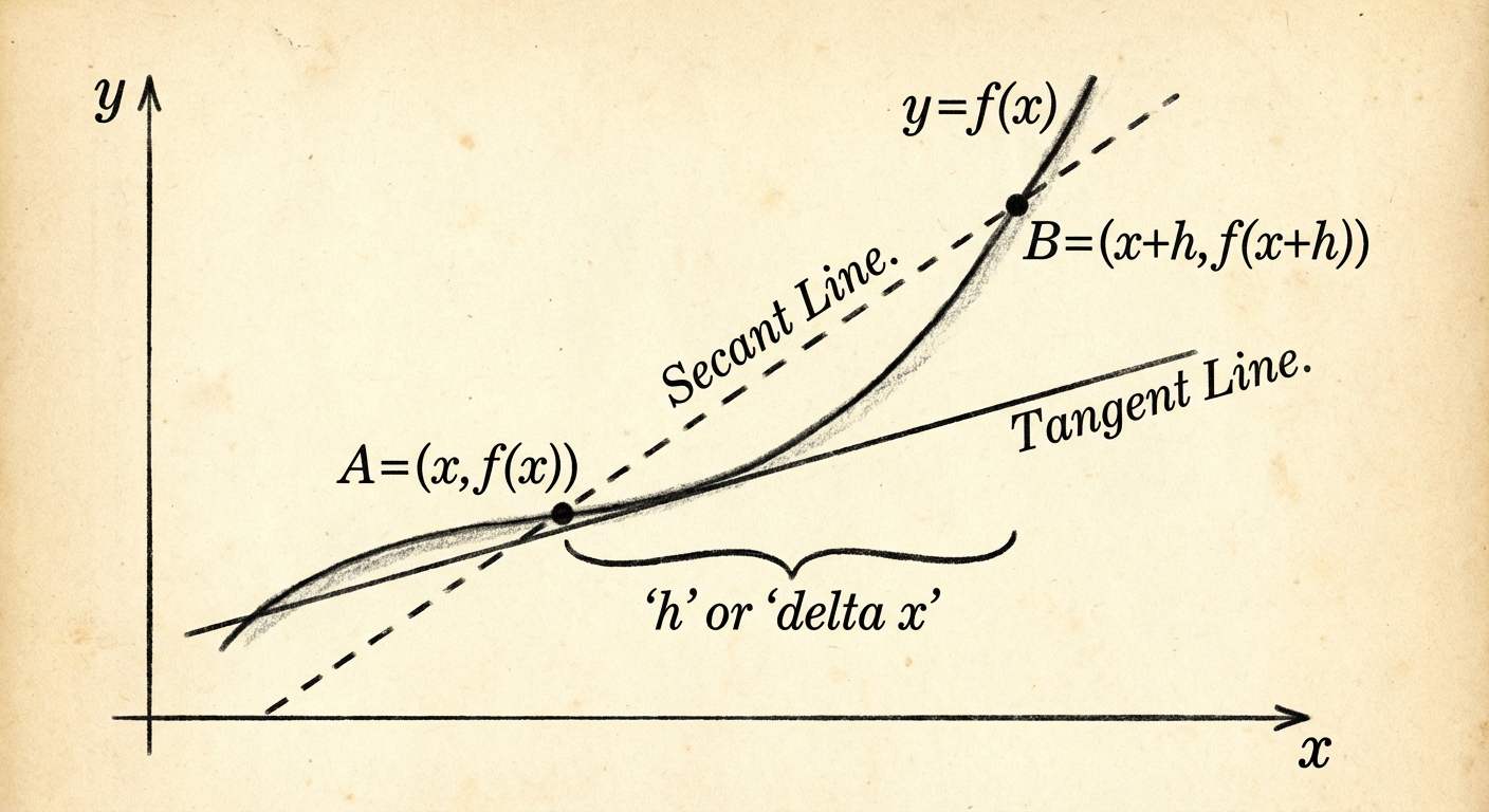
Geometrically, this is the slope of the secant line through the two points
Units matter. If the output is measured in meters and the input in seconds, then the average rate of change is in meters per second.
Instantaneous rate of change (tangent slope)
The instantaneous rate of change at the input value is the slope of the tangent line to the graph at that point (if it exists). Intuitively, if you zoom in far enough near the point, the curve looks almost like a line, and that line’s slope is the instantaneous rate.
You cannot compute an instantaneous rate by setting in the average-rate formula (that would divide by zero). Instead, you use a limit by letting the second input approach the first.
A common setup introduces a small change in input, %%LATEX7%%, so the second input is %%LATEX8%%. The average rate of change from %%LATEX9%% to %%LATEX10%% is
As approaches zero, this expression (if it approaches a single finite number) becomes the instantaneous rate of change.
Worked example: average rate of change
Let
Find the average rate of change from input %%LATEX14%% to input %%LATEX15%%.
Compute the function values:
Apply the formula:
Interpretation: over that interval, the output increases by 5 units per 1 unit of input, on average.
Worked example: building toward instantaneous rate of change
For
approximate the instantaneous rate of change at input value %%LATEX20%% using shrinking values of %%LATEX21%%.
Start with the difference quotient:
Compute:
So
Now choose small values of :
- If %%LATEX27%%, the quotient is %%LATEX28%%
- If %%LATEX29%%, the quotient is %%LATEX30%%
- If %%LATEX31%%, the quotient is %%LATEX32%%
These values approach 4, suggesting the instantaneous rate of change at input 2 is 4.
A key habit is to simplify algebraically before substituting tiny values of . If you substitute too early, rounding can hide the pattern.
Exam Focus
- Typical question patterns:
- “Find the average rate of change on an interval and interpret its meaning (including units).”
- “Approximate the instantaneous rate of change at an input value using nearby values from a table or graph.”
- “Relate average rate of change to secant slope and instantaneous rate of change to tangent slope.”
- Common mistakes:
- Confusing average with instantaneous: if you see “average,” use two points; if you see “instantaneous,” you need a derivative idea.
- Mixing up subtraction order in the secant-slope formula.
- Forgetting units or misreading “per unit of input.”
- Using only left-side or only right-side information when the problem intends an overall instantaneous rate.
Defining the Derivative of a Function
The key idea: a limit of average rates
The derivative makes “instantaneous rate of change” precise by using a limit. Conceptually, you take the average rate of change over a very small interval and see what it approaches as the interval shrinks to zero.
At the input value , the derivative is defined by
This is the limit definition of the derivative.
This definition is foundational: later shortcut rules come from it, and on the AP exam you still need it to reason about differentiability, interpret limits, and handle unusual functions.
Two equivalent limit forms you must recognize
You will commonly see two closely related forms.
1) The “” definition (derivative as a function):
This emphasizes “rise over run.” The numerator is the change in output, and the denominator is the change in input.
2) The alternative definition at a point:
These are equivalent because the substitution
turns one form into the other.
AP multiple-choice recognition tip: You are often asked to identify what derivative a limit represents by matching the structure. For example,
matches the pattern
so it represents the derivative of
at the input value .
Notation reference (all mean “the derivative”)
Calculus notation comes from Newton and Leibniz (and later Lagrange), so you must be fluent in several forms.
| Meaning | Notation | Typical use |
|---|---|---|
| Derivative of the function at an input value | A single slope/rate at one point | |
| Derivative function | A new function giving slope at each input | |
| Shorthand derivative of the output variable | When the output is named | |
| Derivative of output with respect to input | Emphasizes “rate of change,” connected to secant slope ideas like | |
| Operator form | An instruction: “take the derivative of what’s inside” |
Geometric meaning: slope of the tangent line
If the derivative exists at the input value , then it equals the slope of the line tangent to the graph at the point
Once you know the slope, the tangent line equation comes from point-slope form:
This is also the basis of local linearity: near the input value , the function behaves approximately like its tangent line.
Physical meaning: velocity as a derivative
If position is given by a function of time,
then average velocity over a small time interval of length is
Taking the limit as approaches zero gives instantaneous velocity:
The same structure appears in marginal cost, population growth rate, current in circuits, and many other applications.
Worked example: derivative from the definition
Find the derivative function for
using the limit definition.
Start:
Compute:
Substitute and simplify:
Factor and cancel the common factor of :
Now take the limit:
A common misconception is trying to plug in %%LATEX68%% immediately. You must simplify first because the original difference quotient is undefined at %%LATEX69%%.
Worked example: derivative at a specific point (conjugates)
Let
Compute the derivative at input value from the definition.
Start:
Multiply by the conjugate:
Simplify the numerator:
So
Now substitute :
This highlights a recurring theme: the definition often requires algebra (factoring, conjugates) to remove the “division by zero” barrier before evaluating the limit.
Exam Focus
Typical question patterns:
- “Use the limit definition to find the derivative function for a given formula.”
- “Write a limit expression for the derivative at an input value and interpret it as a slope or rate.”
- “Find the equation of the tangent line at an input value using the derivative.”
- “Identify what function (and what point) a limit is differentiating by matching the limit structure.”
Common mistakes:
- Substituting before simplifying.
- Algebraic cancellation errors: you may cancel a factor of %%LATEX79%%, but you cannot cancel an %%LATEX80%% that is added.
- The “point trap” in limits: in
the denominator tells you the approach is %%LATEX82%%, not %%LATEX83%%.
- Confusing %%LATEX84%% (a single number) with %%LATEX85%% (a function).
Estimating Derivatives at a Point
Why estimation matters
On many AP problems you are not given an explicit formula. Instead, you might get a table, a graph, measured data, or an implicitly defined relationship. The derivative still represents slope and instantaneous rate, but you estimate it numerically or visually.
Estimating from a table: difference quotients
To estimate the derivative at an input value from a table, you approximate the limiting process using small intervals around that input.
Forward difference (right-hand estimate):
Backward difference (left-hand estimate):
Symmetric difference (often best when available):
The symmetric difference is often more accurate because it balances behavior from both sides, matching the idea that a derivative depends on approaching from the left and the right.
A strong default strategy is: use the closest data points on either side of the target input value (smallest available step size), unless the data is clearly noisy.
Symmetric difference quotient (structure you’ll see often)
If you need an estimate at input %%LATEX90%% and you have values at inputs %%LATEX91%% and (the points flanking 3), then a natural symmetric estimate is
This is “secant slope across the smallest symmetric interval you’re given.”
Worked example: estimating from a table (symmetric, small step)
Suppose a table gives:
Estimate the derivative at input value .
Using the symmetric difference with step size :
Interpretation: near input 2, the output is increasing at about 6 output units per 1 input unit.
A common pitfall is using a “symmetric” formula when the points are not equally spaced around the target input. If spacing is uneven, you must adjust your approach.
Worked example: estimating from a table (neighbors around the target)
Given the table, estimate the derivative at input value .
| 2 | 4 | 6 | 8 | |
|---|---|---|---|---|
| 10 | 18 | 24 | 35 |
The input value 5 lies between 4 and 6, so use those neighboring points:
Estimating from a graph: tangent line slope
To estimate the derivative at an input value from a graph:
- Locate the point on the curve at that input.
- Sketch the tangent line, the line that best matches the curve’s direction at that point.
- Choose two convenient points on your tangent line (not necessarily on the curve).
- Compute slope using rise over run.
You use points on the tangent line (not the curve) because the derivative is the slope of the tangent line. Zooming in mentally helps: the curve looks straighter near the point, making the tangent estimate more reliable.
One-sided derivatives (and how they affect “does the derivative exist?”)
Sometimes a table or graph shows different behavior from the left and right. Define:
Left-hand derivative:
Right-hand derivative:
The derivative exists at the input value only if both one-sided derivatives exist and are equal.
Worked example: detecting a non-existent derivative from slopes
Suppose from a graph you estimate slopes approaching input value :
- From the left, tangent-like slopes approach about
- From the right, tangent-like slopes approach about
Then the derivative at input 1 does not exist because the left-hand and right-hand rates disagree. The function might still be continuous there, but it is not differentiable.
Exam Focus
- Typical question patterns:
- “Estimate the derivative at an input value from a table using values near the target.”
- “Estimate the slope of the tangent line at a point from a graph.”
- “Use left-hand and right-hand estimates to decide whether the derivative exists.”
- Common mistakes:
- Using points too far from the target input (that gives a coarse average rate of change, not a good instantaneous estimate).
- Claiming a symmetric difference while using unevenly spaced points.
- Computing slope using points on the curve rather than on the tangent line when working from a graph.
- Forgetting that different one-sided behavior means “derivative does not exist,” even if the function value exists.
Differentiability and Continuity
Continuity: no breaks in the graph
A function is continuous at the input value if all three are true:
- is defined.
- exists.
- .
Informally, continuity means no hole, jump, or infinite blow-up at that input value.
Differentiability: a well-defined tangent slope
A function is differentiable at the input value if the limit
exists as a finite real number. Differentiability is stronger than continuity: it requires not only “no breaks,” but also “no sharp behavior” preventing a single tangent slope.
The fundamental relationship (the “Fundamental Theorem of Differentiability”)
Theorem: If a function is differentiable at an input value, then it must be continuous at that input value.
Memory aid: “To be Differentiable, you must first be Continuous.” Think: to be a Dragon, you must be a Creature (but not all creatures are dragons).
The converse is false: a function can be continuous at an input value but not differentiable there.
Why differentiability forces continuity (intuition)
The difference quotient
can only settle to a limit if %%LATEX118%% approaches %%LATEX119%% as approaches zero. A hole or jump prevents that, so the “slope over a tiny interval” cannot stabilize.
Where differentiability fails
A derivative fails to exist at an input value in four common geometric situations.
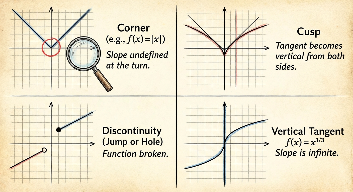
- Discontinuity: hole, jump, or asymptote (not continuous, so not differentiable).
- Corner (sharp turn): left-hand and right-hand slopes are finite but unequal.
- Cusp: slopes approach %%LATEX121%% and %%LATEX122%% from opposite sides (extremely sharp point).
- Vertical tangent: slope becomes infinite (tangent line is vertical), so the derivative is not a finite number.
Examples often used:
- Corner example at input 0:
- Cusp example at input 0:
- Vertical tangent example at input 0:
Worked example: continuous but not differentiable (corner)
Consider
at input value .
The function is continuous there (no break), but the one-sided difference quotients disagree.
For :
For :
Since the left-hand and right-hand limits are not equal, the derivative at 0 does not exist.
Worked example: discontinuity implies not differentiable
Suppose a function has a jump at input value , meaning the left-hand and right-hand limits of the function at 2 are not equal. Then
does not exist, so the function is not continuous at 2. Because differentiability implies continuity, the derivative at 2 cannot exist.
On the AP exam, a complete justification is often as short as:
- Not continuous at input 2
- Therefore not differentiable at input 2
Connecting to tangent lines and motion
Differentiability guarantees a meaningful instantaneous rate.
- If a position function is differentiable at a time value, then instantaneous velocity exists there.
- If the position graph has a corner at that time, it would imply two different instantaneous velocities (from left and right), which is why the derivative does not exist.
Pointwise thinking (a subtle but important habit)
Differentiability and continuity can change from point to point. A function might be differentiable at one input value and not at another, or continuous everywhere but fail to be differentiable at a few corners. Unless a problem explicitly says “for all inputs in an interval,” make your statements at a specific input value.
Comparing concepts table
| Condition | Implies Continuity? | Implies Differentiability? |
|---|---|---|
| Function is differentiable | YES | YES |
| Function is continuous | YES | MAYBE (check corners/cusps/vertical tangents) |
| Function is not continuous | NO | NO (impossible) |
Exam Focus
- Typical question patterns:
- “Is the function continuous or differentiable at an input value? Justify using a graph, table, or the limit definition.”
- “Identify where a function is not differentiable (corner, cusp, vertical tangent, discontinuity) and state the correct reason.”
- “Use ‘differentiable implies continuous’ to make quick conclusions.”
- Common mistakes:
- Assuming “continuous implies differentiable” (false). The absolute value corner is a standard counterexample.
- Confusing a vertical tangent with slope zero; a vertical tangent corresponds to an infinite (undefined) slope, not zero.
- Declaring non-differentiability from a rough sketch without naming the correct cause (AP graders care about the reason: corner vs. cusp vs. discontinuity vs. vertical tangent).