Unit 9 Review: Vector-Valued Functions in AP Calculus BC

Vector-Valued Functions

Vector-valued functions are the bridge between parametric equations and vector calculus. In AP Calculus BC, you are primarily responsible for planar (2D) movement. While parametric equations describe relationships as $x(t)$ and $y(t)$, vector-valued functions package these into a single vector object.

Defining and Differentiating Vector-Valued Functions

Definitions and Notation

A vector-valued function is a function whose domain is a set of real numbers (usually time, $t$) and whose range is a set of vectors. It effectively traces a parametric curve in the plane.

There are two common notations you must recognize:

1. Component Form: $\mathbf{r}(t) = \langle x(t), y(t) \rangle$
2. Unit Vector Form: $\mathbf{r}(t) = x(t)\mathbf{i} + y(t)\mathbf{j}$

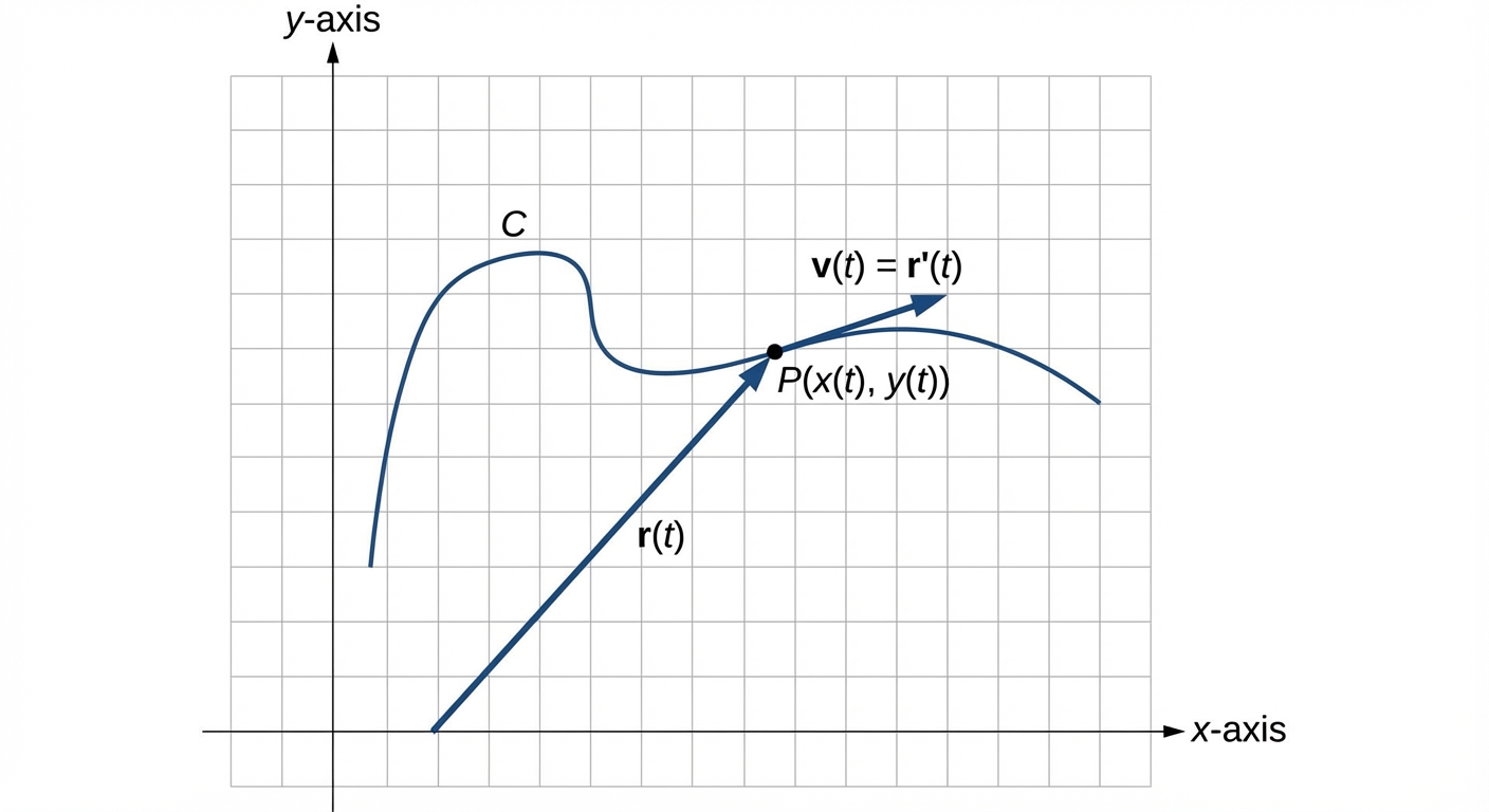
Here, $x(t)$ and $y(t)$ are the component functions. The vector $\mathbf{r}(t)$ represents the position vector starting from the origin $(0,0)$ and pointing to the point $(x(t), y(t))$ on the curve.

Limits and Continuity

Calculus operations on vector-valued functions are performed component-wise (separately for $x$ and $y$).

For a function $\mathbf{r}(t) = \langle f(t), g(t) \rangle$:
$\lim<em>{t \to a} \mathbf{r}(t) = \left\langle \lim</em>{t \to a} f(t), \lim_{t \to a} g(t) \right\rangle$

The function is continuous at $t=a$ if limits exist for both components and equal the function value at that point.

Differentiation

If $x(t)$ and $y(t)$ are differentiable functions, the derivative of the vector-valued function is:

$\mathbf{r}'(t) = \frac{d}{dt}\langle x(t), y(t) \rangle = \langle x'(t), y'(t) \rangle$

Key Geometric Property:
The derivative vector $\mathbf{r}'(t)$ is tangent to the curve at the point corresponding to $t$, pointing in the direction of orientation (motion).

Integration

Integration is also performed component-wise. This applies to both definite and indefinite integrals.

Indefinite Integral:
$\int \mathbf{r}(t) \, dt = \left\langle \int x(t) \, dt, \int y(t) \, dt \right\rangle + \mathbf{C}$
Note: $\mathbf{C}$ is a constant vector $\langle C<em>1, C</em>2 \rangle$, not a scalar.

Definite Integral:
$\int<em>{a}^{b} \mathbf{r}(t) \, dt = \left\langle \int</em>{a}^{b} x(t) \, dt, \int_{a}^{b} y(t) \, dt \right\rangle$

Solving Motion Problems Using Parametric and Vector-Valued Functions

The most common application of vector functions in AP Calculus BC is particle motion in a plane. You are treating the $(x, y)$ coordinates as the position of a particle at time $t$.

Kinematics: Position, Velocity, and Acceleration

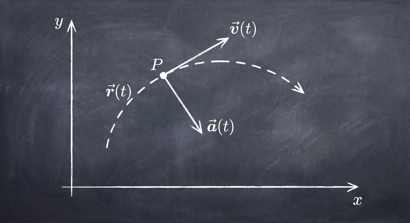
If $\mathbf{r}(t) = \langle x(t), y(t) \rangle$ is the position vector, then:

Speed vs. Velocity

This is a critical distinction in physics and calculus.

• Velocity is a vector (it has direction and magnitude).
• Speed is a scalar (it is the magnitude of the velocity vector).

Formula for Speed:
$Speed = |\mathbf{v}(t)| = \sqrt{(x'(t))^2 + (y'(t))^2}$

Displacement and Distance Traveled

When analyzing motion over a time interval $[a, b]$, we distinguish between how far the particle ended up from where it started (displacement) and how much ground it covered (distance).

1. Displacement

Displacement is a vector representing the net change in position.
$Displacement = \int_{a}^{b} \mathbf{v}(t) \, dt = \langle x(b) - x(a), y(b) - y(a) \rangle$

2. Total Distance Traveled

Distance is a scalar representing the arc length of the path traveled. It is the integral of speed.
$Total \, Distance = \int<em>{a}^{b} |\mathbf{v}(t)| \, dt = \int</em>{a}^{b} \sqrt{(x'(t))^2 + (y'(t))^2} \, dt$

The Fundamental Theorem of Calculus for Vectors

To find the position of a particle at a specific time $t=b$, given the position at $t=a$ and the velocity vector $\mathbf{v}(t)$:

$\mathbf{r}(b) = \mathbf{r}(a) + \int_{a}^{b} \mathbf{v}(t) \, dt$

Broken down by components:

• $x(b) = x(a) + \int_{a}^{b} x'(t) \, dt$
• $y(b) = y(a) + \int_{a}^{b} y'(t) \, dt$

Worked Example: Particle Motion

Problem:
A particle moves in the $xy$-plane so that its velocity vector is given by $\mathbf{v}(t) = \langle t^2, \cos(t) \rangle$. At time $t=0$, the particle is at position $(2, 3)$.

1. Find the speed of the particle at $t=3$.
2. Find the position of the particle at $t=3$.

Solution:

1. Calculating Speed
Step 1: Identify components of velocity at $t=3$.
$x'(3) = 3^2 = 9$
$y'(3) = \cos(3) \approx -0.99$

Step 2: Apply speed formula.
$Speed = \sqrt{(x'(3))^2 + (y'(3))^2} = \sqrt{81 + \cos^2(3)}$
$Speed \approx \sqrt{81 + 0.98} \approx 9.054$

2. Finding Position
Step 1: Use the Fundamental Theorem of Calculus.
$x(3) = x(0) + \int<em>{0}^{3} x'(t) \, dt = 2 + \int</em>{0}^{3} t^2 \, dt$
$x(3) = 2 + \left[ \frac{t^3}{3} \right]_0^3 = 2 + (9 - 0) = 11$

$y(3) = y(0) + \int<em>{0}^{3} y'(t) \, dt = 3 + \int</em>{0}^{3} \cos(t) \, dt$
$y(3) = 3 + [\sin(t)]_0^3 = 3 + (\sin(3) - \sin(0)) = 3 + \sin(3) \approx 3.141$

Final Position: $\mathbf{r}(3) = \langle 11, 3+\sin(3) \rangle$

Common Mistakes & Pitfalls

1. Confusing Velocity and Speed

   • Mistake: Integrating velocity to find total distance.
   • Correction: Integrating velocity gives displacement (net change). Integrating speed (magnitude of velocity) gives total distance.

2. Notation Errors

   • Mistake: Writing speed as a vector or velocity as a number.
   • Correction: Remember: Velocity = $\langle a, b \rangle$ (Vector). Speed = $Number$ (Scalar).

3. Forgetting Initial Conditions (The "Shift")

   • Mistake: Calculating position at $t=b$ simply as $\int_0^b \mathbf{v}(t) dt$.
   • Correction: You must add the starting position vector: $\mathbf{r}(b) = \mathbf{r}(a) + \int_a^b \mathbf{v}(t) dt$.

4. Neglecting the Vector Constant of Integration

   • Mistake: Writing $\int \mathbf{v}(t) dt = \mathbf{r}(t) + C$.
   • Correction: The constant is a vector $+ \mathbf{C}$ or $\langle C<em>1, C</em>2 \rangle$, meaning there is an unknown constant for $x$ and a separate unknown constant for $y$.