Logistic Regression

Logistic regression is usually a variable such as an event or occurence
e.g. did a teen graduate high school or not? Did they go to college or not? Either it happened (1) or it didn’t (0)
is non-linear
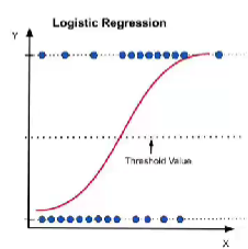
you are looking at the probability of whether a participant attains the Y value, based on what X is. e.g. those in x, y, and z situation won’t, but those in w situation will.
it’s not a matter of what y is bc y is just 1 or 0.
any value
e.g. if x is large, moderate, small
the red line tells us how y changes as x changes
the slop changes over time, which is why it is not linear

Since Y is binary, it has a special distribution it follows: Bernoulli distribution



how we would express this is, “we are predicting the log odds or logits of the outcome or X

In the logit regression equation, the probability of ‘y’ or in this case the logit is p/(1-p), which gives us the odds. From there, you take the natural log of that to get the logit.
The invert it, you take e (exponential), to the power of logit. This gives you the odds. then you plug in the odds as so: odds/(1+odds), which gives you the probability


Maximum Likelihood Estimation is logistic version of the Least squares line
helps to find all the unstandardized coefficients that make the observed data most likely to have occurred.
L = the likelihood/probability of the observed data, given the parameter values/estimates
this is what we want to maximize, which gives us LL
LL = log likelihood
Maximized log-likelihood by doing this: ln(L)
Deviance is calculated by:
minimizing LL by doing this: -2LL
is the same as ln(L), can be an alternative calculation for the same answer
Need to then do a likelihood ratio test
compares the L and LL models using a chi-square test

the reduced deviance is e.g. the version with no predictor, kind of like a control
v.s. your actual experiment/test that you’re writing the paper on
how much the control deviates from your model, compared to the deviance of the full model.

H0 is actually that all slopes will be equal to zero
and then we are not intersted in the constant, we dont report the B0 hypohtheses, so we do not report them.
The last line is the interpretation
I honestly don’t understand why we did the chi square or where the null model comes into play.
df=# of predictors
Pseudo R² is the same as error variance
can also be called the model misfit
gives us different measures (Cox and Snell is one, the other is Nagelkerke, which is more commonly reported)
The Classification Table tells us:
whether the model and the predicted Y successfully predicted what is actually observed
The test of individual Regression Coefficient (Wald)
is the model improved by decreasing the deviance or misfit
sig. is the p-value
The exponential of B
tells us the odds ratio (e^B)
tells us how the odds of Y=1 change for a 1-unit increase in a predictor, holding the other predictors constant
A positive B produces an odds ratio greater than 1, which indicates higher odds
a negative B produces an odds ratio less than 1 (but greater than 0), indicating lower odds
When B=0, the odds ratio is 1 (theyre opposite, in a sense)
this means there is no association between the predictor and the outcome
can never be negative
Makes it to where the odds change by a certain %, this value, as the predictor variable goes up by 1
