Topic 6
Understand ANOVA and Regression as Both Part of the General Linear Model
Regression and ANOVA both aim to explain scores on an outcome or dependent variable
Regression: looks at the associations between continuous variables
ANOVA: looks at the mean group differences
Both are part of the general linear model (GLM): data = model + error
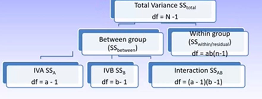
For both, variance is broken up into a few parts:
Regression: regression/residual
ANOVA: between/within
SSregression is based on how different the predicted scores for the individual differ from the mean of the outcome variable. SSbetween is based on how different each group mean is from the grand mean of the DV.
SSresidual is based on how different the predicted scores from the individual are to the actual score on the outcome variable. SSwithin is based on how different individual’s actual scores are from the group mean.
The aim is always to maximise explained variance and minimise unexplained variance.
Understand ANOVA Asks the Question: are the Means Different?
Where regression is about finding associations, ANOVA is about finding the ways in which groups differ.
Example: outcome/DV = reading comprehension; RQ: do reading skills explain reading comprehension scores?
Regression: IV is continuous reading scores
ANOVA: compares different groups of readers based on their reader scores
Designs in ANOVA
Between Groups Variance / Explained Variance
SSbetween = Σn(ȳj – ȳ)^2 : tells us how different each group is from the grand mean
We want to maximise this
ȳj = group mean
ȳ = grand mean
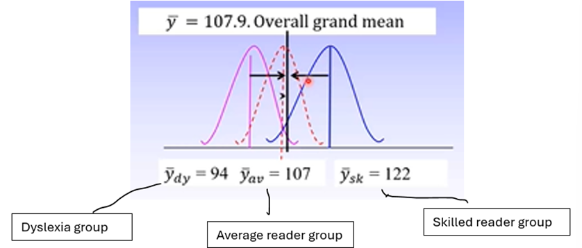
If group means are very different, we expect a large SSbetween
Within Groups Variance / Error Variance
SSwithin = Σn(yij – ȳj)2 tells us how different each individual score is to its group mean
yij = individual score
ȳj = group mean
We want to minimise this
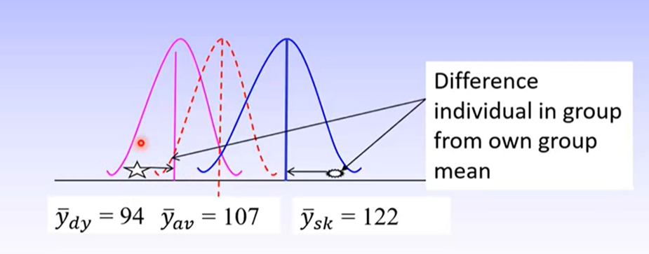
In a ‘good’ model, we would expect very little difference between the individuals score and their group mean, so SSwithin would be very small.
Understand Models are Based on the Number of IVs
Example: Independent one-way ANOVA
IV: reader group (dyslexia, average, skilled)
DV: comprehension score
RQ: Is comprehension score different for different reader groups?
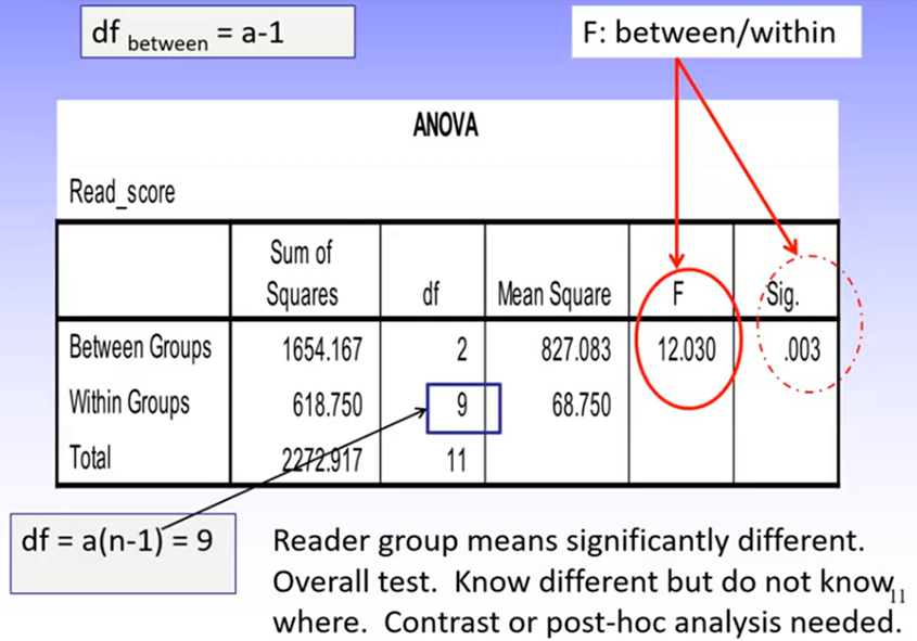
Recall that dfbewteen = a-1, and dfwithin = a(n-1)
a = number of IVs
n = sample size
The ANOVA is an omnibus test; it tells us only if there is a statistically significant effect of the IV, not where this lies.
To know where it occurs, we need to conduct further analyses (contrast analysis or post-hoc analysis)
ANOVA Designs:
Fully independent groups: each participant is in only one group
Fully repeated measures: all participants undertake all conditions
Mixed: a combination of independent and repeated measures
Iin each design, the way variance is explained is the difference between the group mean and the grand mean. What differs between them is the error term:
Independent groups: how different each participants score is from their own group mean
Repeated measures: reduces individual differences and therefore the error term, because the same participants are in all groups
Error Terms in ANOVA Designs
Independent Groups: within group error includes:
Random error
Measurement error
Individual differences
Repeated Measures: within group error includes:
Random error
Measurement error
Does not include individual differences because these can be controlled for, which reduces the size of the error term
Example: repeated measures t-test
DV: score on maths test
IV: time; before and after maths program intervention was administered
Results
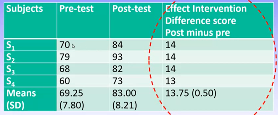
Can see there is a similar amount of change between pre- and post-test for all students.
While the child with the best pre-test score also had the best post-test score, they improved by the same amount as everyone else
In RM ANOVAs, we can statistically control for individual differences.
SSas/ overall error = Σ(ȳai - ȳj)2 : how different each score is from its group mean
SSubjects = aΣ(ȳa - ȳt)2 : how different the individual subjects mean (across conditions) is from the group mean
SSwithin = SSas – Sssubjects: tells us how different individual subject scores are to the group mean while controlling for individual differences
The Model of Factorial ANOVA
Factorial ANOVAs:
Always have 1 DV and more than 1 IV
Ask are the means different?
Produce a main effect, which depicts the influence of the IV without controlling for other IVs in the analysis
May produce an interaction effect, which depicts the influence of one IV on the score on the DV, conditional on the level of the second IV
Like a moderator in regression
Example: 2(task difficulty: easy, hard) × 2 (driver group: has violations, does not have violations) × 2 (Incentive: incentive, no incentive) design
Driver group: between groups
Task difficulty and incentive: repeated measures
This design contains 3 IVs. This introduces higher order effects that make the analysis more complicated to interpret.
While we could use a series of smaller ANOVAs (e.g., 2 2x2 ANOVAs), this is a bad idea because:
It reduces statistical power
It disallows us to interpret the 3-way interaction
Hypotheses
Easy condition:
For drivers with no violations, accuracy was not expected to differ between incentive conditions
For good drivers, accuracy was expected to be better in the incentive than non-incentive condition
Hard condition:
The incentive will provide no advantage in detecting difficulty objects for either driver group
The group with driving violations will have poorer accuracy in all conditions than good drivers
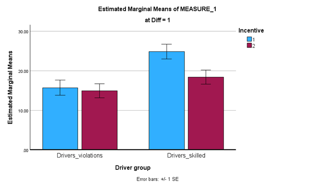
Graphically, if these hypotheses wee confirmed, the results would look a bit like:
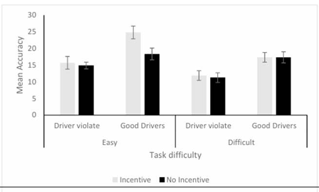
Results:
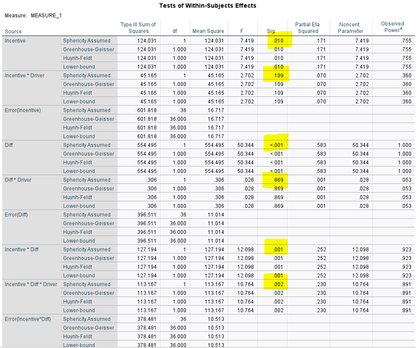
These results indicate:
There is a sig three-way interaction
There is a sig 2-way interaction between incentive and task difficulty
There is no sig 2-way interaction between task difficulty and driver group, or between incentive and driver group
There are 3 sig main effects
Because there is a sig three-way interaction we need to interpret simple effects analyses
Look at multivariate and univariate tests for these
Multivariate tests: compare beginning with between-groups factors
Univariate tests: compare beginning with repeated-measures factors
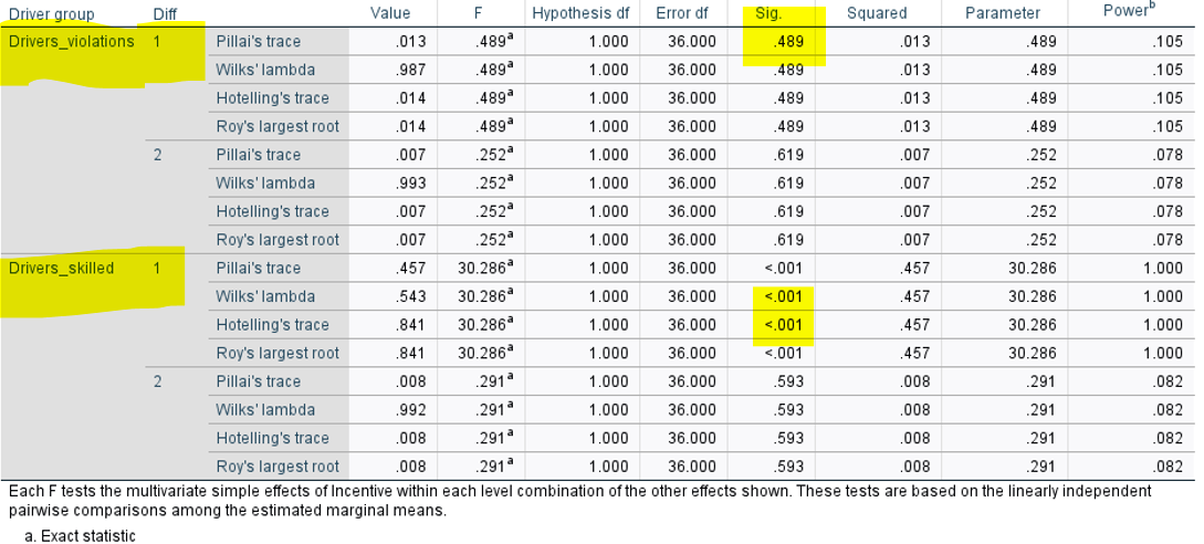
Difficulty 1 = easy task, 2 = hard task (from the way we input it in SPSS)
H1 supported (relevant p nonsig)
H2 supported (relevant p sig)
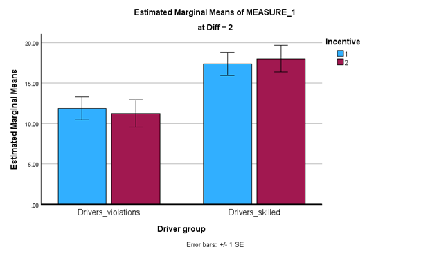
H3 proposed that there would be no difference in performance between incentive and no incentive conditions for either good or bad drivers in the hard condition
Expect the top of the bars between incentive conditions for good and bad drivers alone to be pretty similar in height
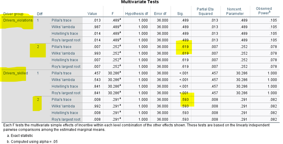
H3 supported (both relevant ps nonsig)
if one was nonsig and one was sig, could say H3 is rejected or partially supported based on the wording of the hypothesis
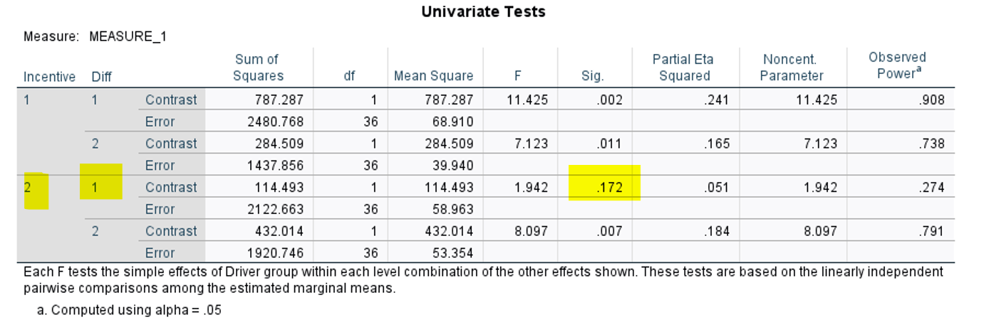
H4 is not supported, because all p’s would need to be sig. because one is not, it is not fully supported.
How Factorial ANOVAs Work
Can see there is only one error term produced, which is generated using the interaction means
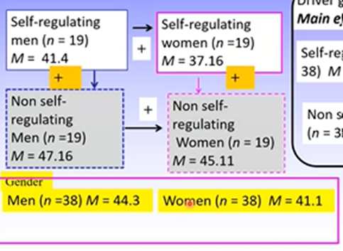
Main Fffects in Factorial ANOVAs
Main effects are the independent influence for one IV on the DV
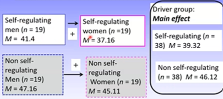
Obtaining the error term for a factorial ANOVA for independent groups is similar to a one-way independent groups ANOVA.
Investigates how different the score for the individual is from their group mean
We use the interaction group means for this as there are several IVs, which allows for these multiple IVs to be accounted for
Interaction Effects of Factorial ANOVAs
Interaction effects: the score on the DV is determined by membership in more than one group, so is a conditional effect
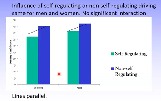
Graphs can indicate whether an interaction effect exists. Here, there is no interaction because the lines between the bars are parallel.
Any difference in group means is not due to interaction effects
How we know if an interaction is 2-way or 3-way:
A 2-way interaction occurs when the outcome under one main effect is conditional on another factor
A 3-way interaction occurs when a 2-way interaction is itself conditional on another factor.
Understand Different Types of Interactions
Example:
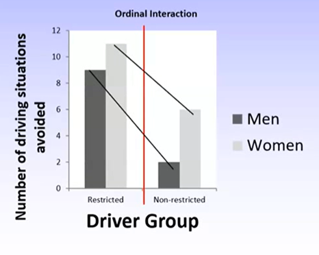
Restricted group: women report more driving difficulties than men
Non-restricted group: there are fewer overall reports of driving difficulty but women report more difficulties than men still
Importantly, there seems to be a difference in the magnitude of the difference between men and women between the two groups – this indicates an interaction effect.
A significant interaction occurs when the pattern for men and women differs based on whether they’re part of the restricted or non-restricted group.
An ordinal interaction is explained by the magnitude or size of the difference for men and women between groups.
In this example, there is a smaller difference between men and women in the restricted group than non-restricted group
A disordinal interaction occurs when the effect of one IV differs at the level of the second IV and the direction or effect differs.
A more powerful kind of effect
Means we cannot interpret any sig main effects – this is why we must examine any interactions/ higher order effects first before considering the significance of any other effects
This is an example of a disorderly interaction with respect to gender. This is because the direction of the effect between gender and DV changes based on the level of the second IV
Performing and Interpreting Simple Fffects Analyses Based on Research Questions
Where there are disordinal interactions between one or more IVs:
Interpret the interaction first
Cannot interpret main effects associated with the crossover
Where there are ordinal interactions:
Can interpret main effects if the interaction is one of magnitude (not direction)
Must ensure the sig interaction is not an artefact of measurement: caused by a few extreme scores in one group that promotes an interaction effect that isn’t really there
Check distributions to ensure this isn’t the case
Regardless of the interaction, further analyses must be conducted where there is a significant interaction.
For all research, it is required to have research questions and hypotheses that need to be answered.
One of the proposed reasons for the replication crisis was because people interpreted their data first and determined RQs after – called p-hacking
It is a researchers job to provide evidence that supports or fails to support their proposed hypotheses.
Can still report non-hypothesised effects, but only as exploratory findings
Simple effects analyses are also known as simple main effects analyses. This is one way to evaluate significant interaction terms.
Allows us to investigate the influence of one IV at each level of the second IV
Examined using multivariate and univariate tests
Analysis of Significant Interactions Where There are More Than 2 Levels of the IV
Example: 2 x 3 fully RM design
DV = mean correct reaction time
IV1 =number of distractors (4, 8, 16)
IV2 = target presence (present, absent)
RM: all participants undertake all conditions
Hypotheses:
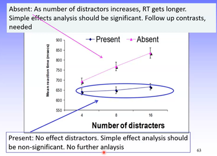
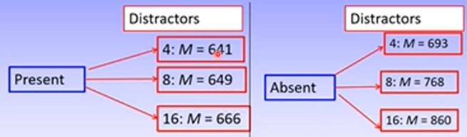
Target present: no effect of distractors
Target absent: 1) mean current response time for 8 distractors will be greater than correct response time for 4 distractors. 2) mean current RT for 16 distractors will be greater than correct RT for 8 distractors
Therefore, were expecting different effects depending on whether the target is present or absent, so there should be a significant interaction
Results
Main effects:
Number of distractors: sig
Target presence: sig
Interaction: sig
As the hypotheses were based on a sig interaction, this is a good sign.
Simple Effects Analyses
Target present: nonsig, supports hypothesis
Target absent: sig, may support hypothesis but need to confirm the direction.
Contrast Analysis: can confirm where exactly the significant difference lies.
Ignore target present as this was nonsignificant
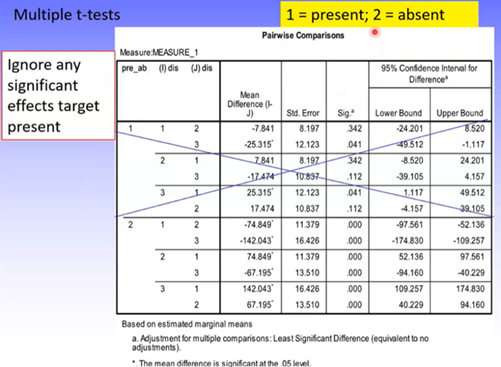
1 = 4 distractors
2 = 8 distractors
3 = 16 distractors
Can see that:
Target absent: there’s a sig difference in RT between 4 and 8 distractors
Target absent: there’s a sig difference in RT between 8 and 16 distractors
Outcome
Regardless of the number of distractors presented for the target present condition, RT was the same.
In target absent condition, as number of distractors increased so did RT.