Chapter 9: Monopoly
Characteristics and Objectives of Pure Monopoly
Focus: Understand pure monopoly concepts, price and output determination, price discrimination, and regulation.
LO1: Key learning objectives include identifying monopoly characteristics, barriers to entry, how price and output are determined, how price discrimination can occur, and regulatory options.
Introduction to Pure Monopoly: Characteristics
Single seller: A sole producer controls the entire market supply.
No close substitutes: Product is essentially unique.
Price maker: Monopoly has control over the price; can set price rather than take market price.
Blocked entry: Strong barriers prevent new entrants from competing.
Non-price competition: Advertising and public relations are often used to differentiate the product rather than competing on price.
LO1: A pure monopoly means that there is only one producer of the good with no close substitutes being produced by any other firms. Since the firm is the industry, they have control over the price that is charged for their good. Monopolies are created and sustained due to strong entry barriers which makes it very difficult for new firms to enter the industry. There is very little non-price competition since there are not any rival firms. There is some non-price competition which merely meant to increase the demand for the good.
Examples of Monopoly
Public utilities: Natural gas, electric, water (typical near-monopoly sectors due to capital intensity and regulatory structure).
Near monopolies: Intel (founded 1968, historically dominant in several microprocessor markets), Wham‑O (toy manufacturer with dominant niche position), professional sports teams (monopolistic franchises in their local markets).
Barriers to Entry
Definition: A barrier to entry is any factor that keeps firms from entering an industry.
Types of barriers:
Economies of scale (graphically shown as ATC falling with higher output, leading to lower average costs at larger scales).
Legal barriers: Patents and licenses.
Ownership of essential resources.
Pricing strategies (e.g., pricing that deters entry).
Economies of Scale (Illustration)
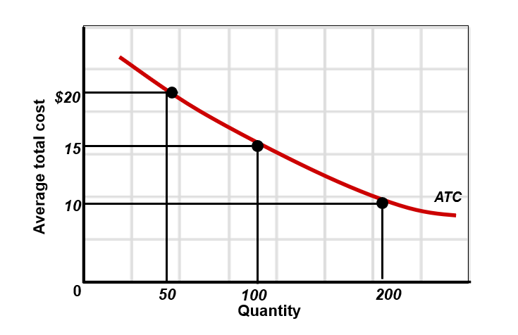
Concept: Average total cost (ATC) declines as output increases due to economies of scale, encouraging a single large producer.
Example values (illustrative): ATC can fall from higher levels as output expands, reflecting economies of scale (e.g., ATC declining as quantity rises from 50 to 200 units).
LO1:Barriers to entry in monopolistic industries include economies of scale, where large firms can produce at the lowest cost, making it inefficient for new firms to enter (e.g., public utilities as natural monopolies, often regulated by the government). Legal barriers include patents (exclusive rights for 20 years to encourage innovation) and licenses (government grants to limit service providers, e.g., radio, TV, taxi companies). Control of essential resources can block entry (e.g., Inco with nickel, DeBeers with diamonds, sports leagues with stadiums). Strategic barriers include predatory pricing, exclusive contracts, and withholding key information (e.g., Dentsply limiting distributors, Microsoft restricting access to its source code).
Monopoly Demand
The monopolist is the industry: The market demand curve is the monopolist’s demand.
Demand is downward sloping: As price falls, quantity demanded rises.
Marginal revenue (MR) is less than price (P): Because selling an additional unit requires lowering the price on all previous units.
LO1: A downward-sloping demand curve and MR < P are fundamental characteristics of monopoly pricing.
The following analysis of monopoly demand makes 3 assumptions:
1) Monopoly is secured by patents, economies of scale or resource ownership2) The firm is not regulated by the government
3) The firm is a single price monopolist it charges the same price for all units of output
Revenue and Cost Data: A Monopolist’s Table (Structure and Implications)
Key components:
Quantity of Output (Q)
Price (Average Revenue, AR, which equals Demand price at that Q)
Total Revenue (TR) = Q × P
Marginal Revenue (MR) = ΔTR/ΔQ
Average Total Cost (ATC)
Total Cost (TC) = ATC × Q
Marginal Cost (MC)
Profit = TR − TC
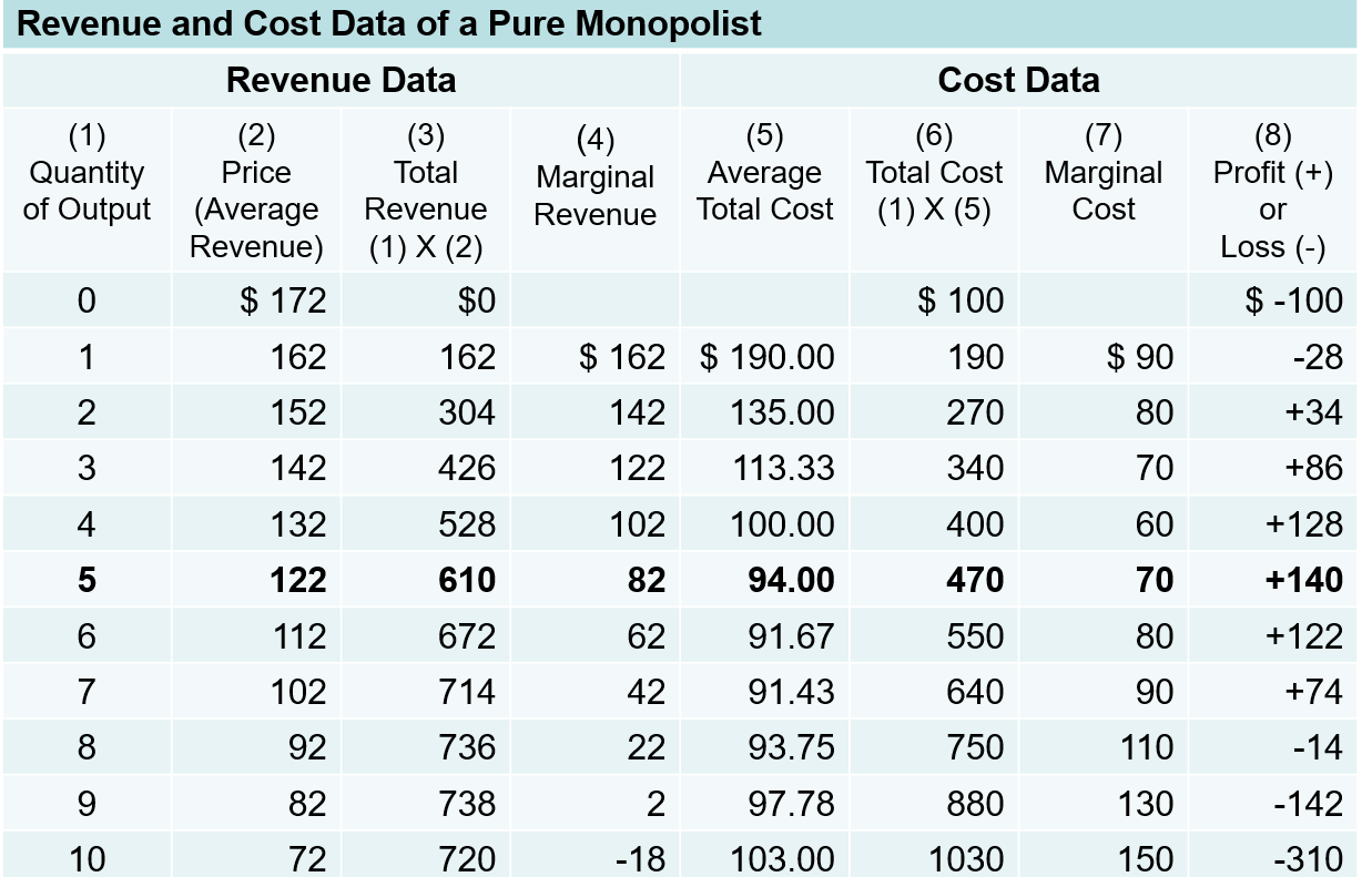
LO1: Price will exceed marginal revenue because the monopolist must lower the price to sell the additional unit. The lower price is applied to all of the units being produced, not just the last unit, thereby causing marginal revenue to be less than price
All customers face the same price at a given output if there is single pricing (no price discrimination in this context).
D, MR curves: Demand is downward sloping; MR lies below the demand curve.
LO1: Monopoly price is set where MR < P; the monopolist must choose a price based on elasticity of demand.
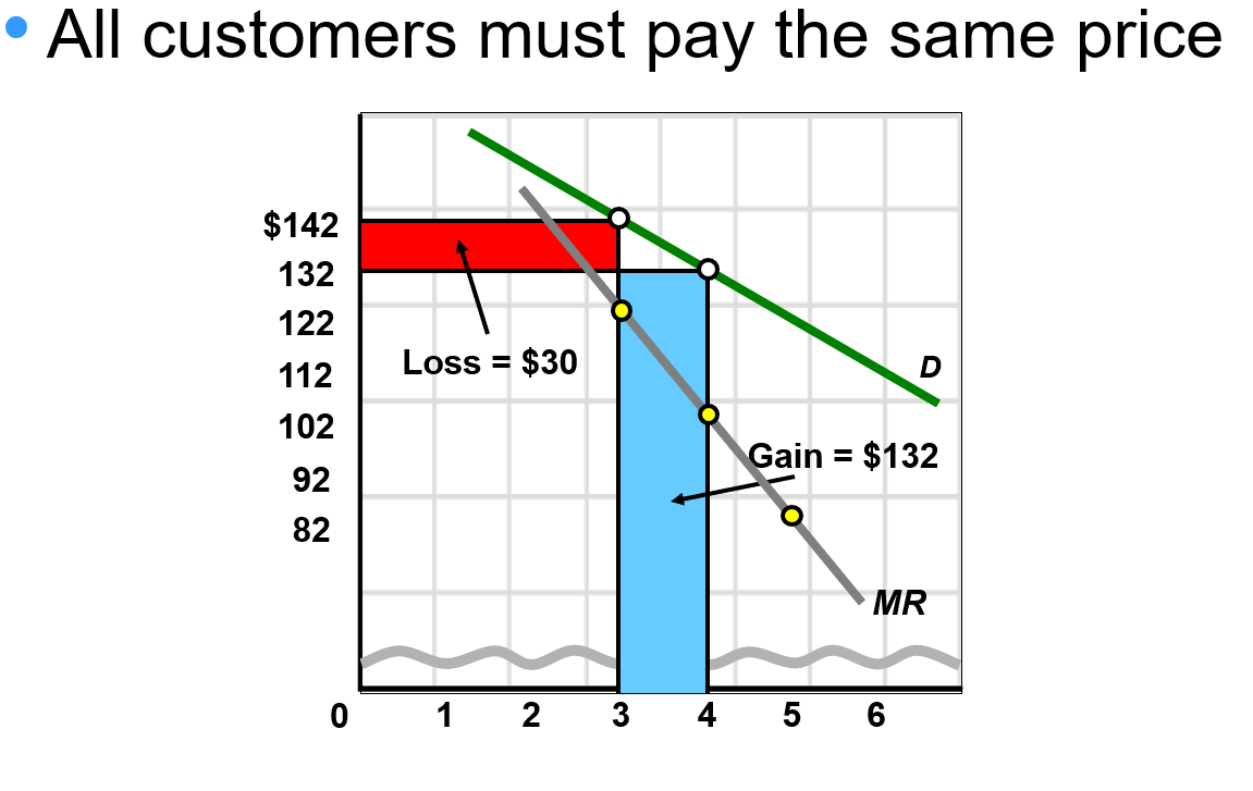
This graph shows the demand and marginal revenue for a pure monopolist. Because it must lower price on all units sold in order to increase its sales, an imperfectly competitive firm’s marginal-revenue curve (MR) lies below its downsloping demand curve (D).
Marginal Revenue and Pricing Power
Key relationships:
MR < Price (P) for a downward-sloping demand curve.
Monopolist is a price maker, not a price taker.
Prices are set in the elastic portion of the demand curve to maximize profits.
LO2: MR is less than price after the first unit sold. A price maker is a firm with pricing power, which is the ability of the firm to set its own price. The monopolist avoids setting the price in the inelastic range of demand.
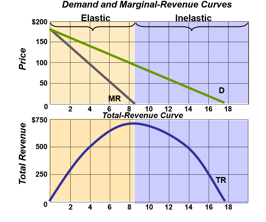
Demand, Marginal & Total Revenues (Conceptual)
TR (Total Revenue) rises at a decreasing rate in the elastic region of demand where MR (Marginal Revenue) > 0 when PED > 1.
TR is maximized when MR = 0 when PED = 1.
In the inelastic region (PED <1), TR falls because MR < 0.
MR curve lies below the downward-sloping demand curve because the monopolist must lower the price on all units to sell more.
Key takeaway: Elastic → MR positive → TR rising; MR = 0 → TR max; Inelastic → MR negative → TR falling.
Steps for Graphical Profit Maximization in Pure Monopoly
Step 1: Determine the profit-maximizing output by finding where MR = MC.
Step 2: Determine the profit-maximizing price by extending a vertical line from the output in Step 1 up to the monopolist’s demand curve (to obtain P).
Step 3: Determine economic profit (if any) using one of two methods:
Method 1: Profit per unit = Price − ATC at the MR = MC output; Total profit = (Price − ATC) × (MR = MC output).
Method 2: Monopoly profit = TR − TC at the output where MR = MC.
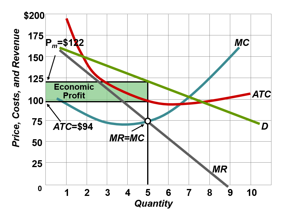
Price, Costs, and Revenue (Illustrative Graph)
At the profit-maximizing output, MR = MC intersects the demand curve, yielding a price (Pm) and output (Qm).
Economic profit is the area where Price exceeds ATC, times the quantity:
Profit = (Pm − ATC) × Qm, provided Pm > ATC(Qm).
Example annotation from slide: Pm = $122, ATC at Qm equals $94 (illustrative), leading to positive economic profit.
The graph below demonstrates profit maximization by a pure monopolist. The pure monopolist maximizes profit by producing at the MR = MC output, here Qm = 5 units. Then, as seen from the demand curve, it will charge price Pm = $122. Average total cost will be ATC = $94, meaning that per unit profit= (Pm – ATC) and total profit = 5 X (Pm - ATC). Total economic profit is thus represented by the green rectangle.
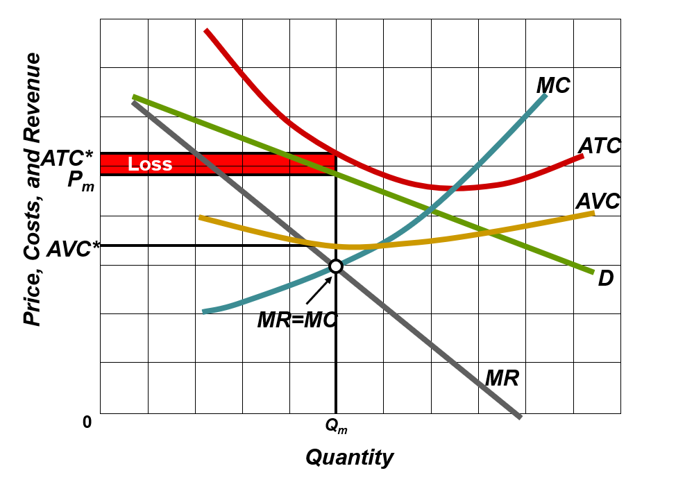
Misconceptions About Monopoly Pricing
Common misconceptions include:
Monopoly pricing means the highest possible price (which ignores demand elasticity and the effect on quantity sold).
Profit is per unit; total profit depends on quantity sold.
Monopolies may incur losses depending on the cost structure and demand.
LO2: It’s important to distinguish per-unit profit from total profit and to recognize that losses can occur even with high prices if costs are too high or demand is too low. The monopolist does not charge the highest possible price because the monopolist “can’t sell much output at that price and profits are too low”. The monopolist is interested in “total profit, not per unit profit”. There is always the possibility that the monopolist will earn losses. Monopolists are not protected from changes in demand.
Economic Effects of Monopoly
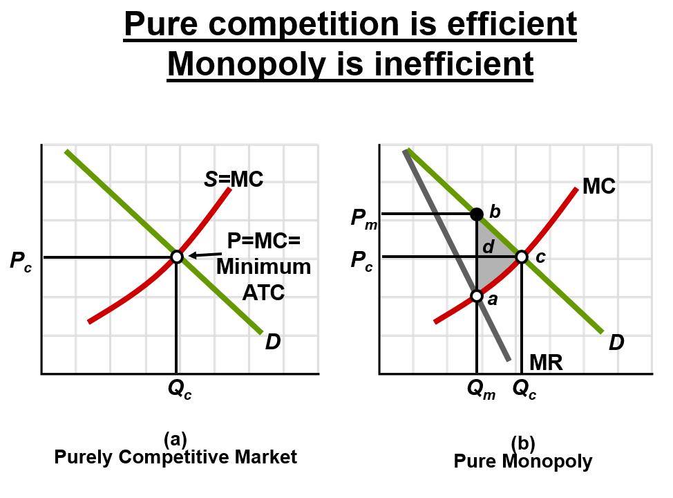
Compared to a purely competitive market, monopoly tends to be inefficient:
Income transfer: Consumers pay higher prices, transferring surplus to the monopolist.
Cost inefficiencies: Difficulties in comparing monopoly with perfect competition due to scale and market power.
Economies of scale: Large-scale production may create efficiency but can also entrench monopoly power.
X-inefficiency: Firms may produce above minimum cost due to lack of competitive pressure.
Rent-seeking expenditures: Resources spent to maintain and secure monopoly power (e.g., lobbying).
Technological progress: Evidence is mixed on whether monopolies spur or hinder innovation.
LO3: In a purely competitive industry, entry and exit of firms ensures that price (Pc) = MC = min. ATC at Qc output. Both productive efficiency (P = minimum ATC) and allocative efficiency (P = MC) are obtained (here at Qc).
In pure monopoly, the MR curve lies below the demand curve. The monopolist maximizes profit at output Qm, where MR = MC, and charges price Pm. Thus, output is lower (Qm rather than Qc) and price is higher (Pm rather than Pc) than they would be in a purely competitive industry. Monopoly is inefficient since output Qm < Qc & P > min. ATC at Qc (productive inefficiency) and P > MC (Allocative inefficiency). Monopoly creates an efficiency loss (here triangle abc). There is also a transfer of income from consumers to the monopoly (here rectangle PcPmbd).
X-Inefficiency (Concept)
X-inefficiency arises when a firm produces at a higher cost than necessary due to lack of competitive pressure.
Illustration: ATC curves can be higher than the minimum ATC even at output levels where competitive firms would operate at minimum ATC.
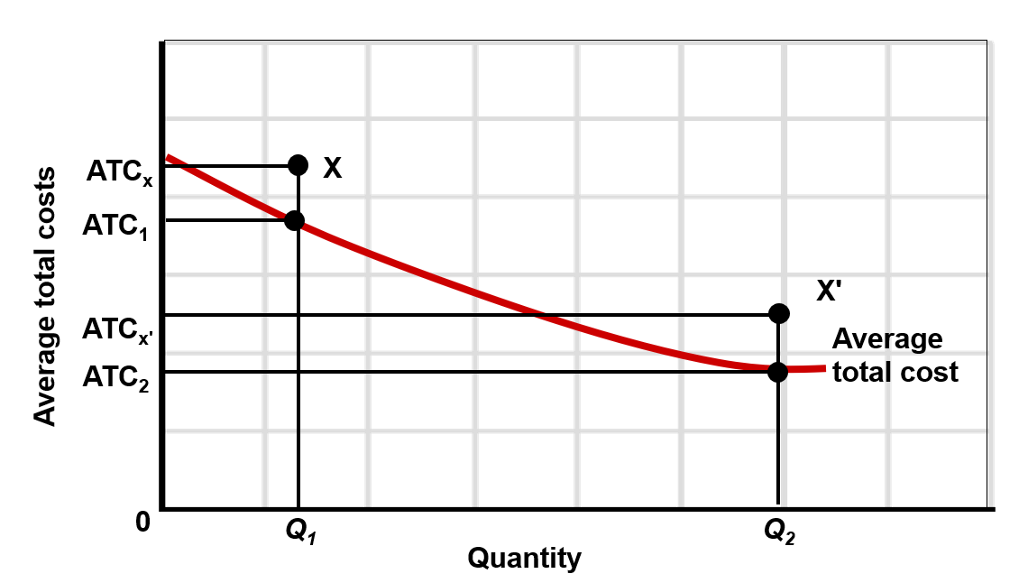
LO3: The average-total-cost curve (ATC) is assumed to reflect the minimum cost of producing each particular level of output. Any point above this “lowest-cost” ATC curve, such as X or X', implies X-inefficiency: operation at a greater cost than the lowest cost possible for a particular level of output.
Price Discrimination by Monopolists
Definition: Charging different buyers different prices not based on differing costs.
Conditions for success:
Monopoly power (ability to set prices).
Market segmentation (the ability to segment buyers by willingness to pay).
No resale (customers who pay a lower price cannot resell to those charged higher prices).
Examples of Price Discrimination
Business travel, electric utilities, movie theaters, railroad companies.
Coupons and other price-reducing devices to segment markets (e.g., student discounts).
International trade price discrimination across borders.
LO4: Business travelers have relatively inelastic demand due to no time to shop around and wait. Also, the firm is paying for this business trip and whenever someone else pays for your consumption, you are not as concerned about the price. Therefore, airlines charge business travelers higher prices than the rest of the population. Hotels will charge the business traveler higher rates than the rest of the population.
Movie theaters charge higher prices for the evening show than for an afternoon matinee. This is because those going to the matinee are more price sensitive than the rest of the population. Those going to the matinee may be retired, families with children, or unemployed people. Those going to the evening show often consider this a special event and are willing to pay full price or perhaps they are too busy working during the day to go to a matinee. This group will be less price sensitive. Also, movie theaters charge adults a higher price than children even though it costs the same amount to show a movie to an adult as to a child. This effort will bring in more people and more revenue because otherwise a family might not be able to afford to bring all members to the show.
Those who have the time and take the time to clip coupons and manage coupons are the price sensitive group. Those who do not take the time are those willing to pay regular price.
Graphical Analysis of Price Discrimination
Conceptual diagram shows separate segments with different demand elasticities (e.g., more elastic segment like students vs. inelastic segment like small businesses).
With discrimination, monopolists may produce more output and earn higher profits compared with single-price monopoly.
Economic profits can be enhanced through segment-specific pricing while still earning profits across segments.
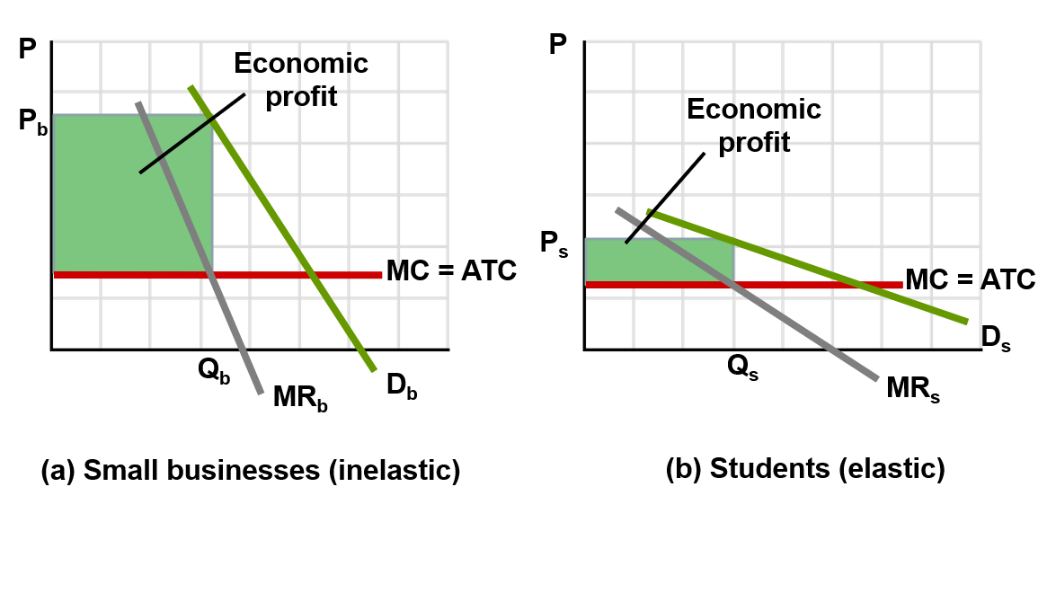
LO4: The price-discriminating monopolist represented here maximizes its total profit by dividing the market into two segments based on differences in elasticity of demand. It then produces and sells at the MR = MC output in each market segment. (For visual clarity, average total cost (ATC) is assumed to be constant. Therefore MC equals ATC at all output levels.) (a) The firm charges a higher price (here, Pb) to customers who have a less elastic demand curve and (b) a lower price (here, Ps) to customers with a more elastic demand. The price discriminator’s total profit is larger than it would be with no discrimination and a single price.
Assessment and Policy Options for Monopolies (Public Policy Context)
Antitrust laws: Seek to promote competition and prevent abuses of monopoly power.
Break up the firm: Structural remedies to reduce market power.
Regulate it: Government imposes controls on price and output (direct regulation).
Ignore it: Allow time and markets to adjust and potentially erode monopoly power naturally.
LO3: When monopoly power results in an adverse effect upon the economy, the government may choose to intervene on a case-by-case basis using antitrust laws. If the government feels that it is more beneficial to society to have a monopoly, then government will regulate it. Although there are legitimate concerns of the effects of monopoly power on the economy, monopoly power is not widespread. While research and technology may strengthen monopoly power, overtime it is likely to destroy monopoly position.
Regulated Monopoly: Natural Monopolies and Pricing Rules
Natural monopolies: Industries where a single firm can supply the entire market at lower cost than multiple firms (e.g., utilities).
Socially optimal price: Set price equal to marginal cost (P = MC) to maximize total welfare.
Fair return price: Set price equal to average cost (P = ATC) to ensure the regulator allows a normal return on investment.
When monopoly power adversely affects the economy, governments, especially in the U.S. for natural monopolies, may intervene. Regulators face a dilemma: setting a socially optimal price () is most efficient but can lead to firm losses requiring subsidies, while a fair-return price () ensures normal profit but sacrifices allocative efficiency.
Regulated Monopoly: Graphical Illustration (Key Points)
Demand (D) intersects with marginal cost (MC) and ATC curves.
Regulated price schemes include socially optimal price (P = MC), fair-return price (P = ATC), and other regulatory constructs.
In the graph, the monopoly price (Pm) and regulated prices (Pf, Pr) are indicated at different outputs; the regulator’s aim is to choose a price path that aligns with social welfare goals.
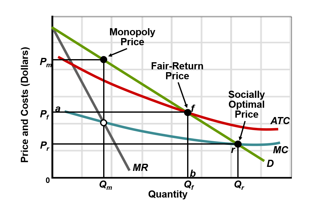
LO5: The socially optimal price Pr, found where D and MC intersect, will result in an efficient allocation of resources but may entail losses to the monopoly (P< ATC at Qr). The fair-return price, Pf, will allow the monopolist to break even (P=ATC) but will not fully correct the underallocation of resources (P > MC).