Math 134/Unit 6.Week6 Exponential Growth and Decay, Linearization, Continuity, Intermediate Value Theorem, and Extrema

Overview of Differential Calculus Topics

• Transition from Skill Building to Application:
  • Unit 5 focused on techniques for finding derivatives of all sorts of functions, including the product rule, quotient rule, chain rule, implicit differentiation, and logarithmic differentiation.
  • Unit 6 applies derivative techniques to analyze mathematical models and function properties, encompassing:
  • Natural laws of growth and decay
  • Linear approximations (tangent line approximations)
  • Continuity of a function $f(x)$ at a point $x = a$
  • The Intermediate Value Theorem (IVT)
  • Maxima and minima of functions

Natural Laws of Growth and Decay

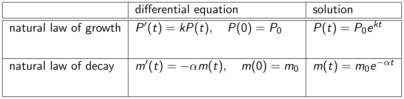
• Differential Equations and Solutions:
  • Natural Law of Growth:
  • Differential Equation: $P'(t) = kP(t)$ with initial condition $P(0) = P_0$
  • Solution: $P(t) = P_0 e^{kt}$
  • Relative Growth Rate: $\frac{P'(t)}{P(t)} = k$
  • Natural Law of Decay:
  • Differential Equation: $m'(t) = -\alpha m(t)$ with initial condition $m(0) = m_0$
  • Solution: $m(t) = m_0 e^{-\alpha t}$
  • Half-Life Formula: $t_{\frac{1}{2}} = \frac{\ln(2)}{\alpha}$

• Application Problems and Solved Questions:
  • Question 6.1: E. coli Growth:
  • Problem Statement: The growth of E. coli bacteria in a petri dish can be described by a natural law of growth. The relative growth rate is $\frac{1}{20}$ per minute, and the initial condition is $P(0) = 60$ cells. Write down the law of natural growth for the E. coli population and find its solution. Find the time at which the bacterial population will have doubled (doubling time).
  • Differential Equation: $P'(t) = \frac{1}{20}P(t)$ with $P(0) = 60$
  • Solution: $P(t) = 60 e^{\frac{1}{20}t}$
  • Doubling Time Calculation:
    • Set $P(t) = 2 \times 60 = 120$
    • $60 e^{\frac{1}{20}t} = 120 \implies e^{\frac{1}{20}t} = 2$
    • $\frac{1}{20}t = \ln(2) \implies t = 20 \ln(2) \text{ minutes}$
  • Question 6.2: Exponential Decay:
  • Problem Statement: Strontium 90 has a half-life of $28$ days. Write down a model for the radioactive decay of strontium with an initial mass of $m_0$
  • Decay Rate Constant $\alpha$ Calculation:
    • $28 = \frac{\ln(2)}{\alpha} \implies \alpha = \frac{\ln(2)}{28}$
  • Differential Equation: $m'(t) = -\left(\frac{\ln(2)}{28}\right) m(t)$ with $m(0) = m_0$
  • Solution Model: $m(t) = m_0 e^{-\left(\frac{\ln(2)}{28}\right)t} = m_0 \left(\frac{1}{2}\right)^{\frac{t}{28}}$

Linear Approximations and Linearization

• Theoretical Foundations:

  • The tangent line to the graph of $y = f(x)$ at a given point $(a, f(a))$ provides a linear approximation to the function for $x$ near $a$
  • Linearization Formula: The function $L(x) = f(a) + f'(a)(x - a)$ is called the linearization of $f$ at $a$

• Linearization Questions and Applications:

  • Question 6.3: Linearization of Polynomial Function:
  • Problem Statement: Find the linearization $L(x)$ of the function $f(x) = x^4 + 3x^2$ at $a = -1$
  • Step 1: Compute $f(-1) = (-1)^4 + 3(-1)^2 = 1 + 3 = 4$
  • Step 2: Compute derivative $f'(x) = 4x^3 + 6x$
  • Step 3: Compute slope at $a = -1$: $f'(-1) = 4(-1)^3 + 6(-1) = -4 - 6 = -10$
  • Step 4: Construct $L(x) = 4 + (-10)(x - (-1)) = 4 - 10(x + 1) = -10x - 6$
  • Answer Options:
    • (a) $L(x) = -5x + 3$
    • (b) $L(x) = -10x + 6$
    • (c) $L(x) = -10x - 6$ (Correct)
    • (d) $L(x) = -5x - 3$
  • Question 6.4: Linear Approximation of Exponential Function:
  • Problem Statement: Consider the function $f(x) = e^{-(x-2)^2}$
    1. Find the linear approximation $L(x)$ at the point $a = 1$
    2. Use the linearization to approximate the value $e^{-0.81}$
  • Solution Part 1:
    • Evaluate $f(1) = e^{-(1-2)^2} = e^{-(-1)^2} = e^{-1}$
    • Differentiate $f'(x) = e^{-(x-2)^2} \cdot (-2(x-2)) = -2(x-2)e^{-(x-2)^2}$
    • Evaluate slope $f'(1) = -2(1-2)e^{-1} = 2e^{-1}$
    • Form linearization $L(x) = e^{-1} + 2e^{-1}(x - 1) = e^{-1}(1 + 2x - 2) = e^{-1}(2x - 1)$
  • Solution Part 2:
    • Identify $x$ such that $-(x-2)^2 = -0.81 \implies (x-2)^2 = 0.81 \implies x - 2 = -0.9 \implies x = 1.1$
    • Approximate value: $f(1.1) \approx L(1.1) = e^{-1}(2(1.1) - 1) = e^{-1}(2.2 - 1) = 1.2e^{-1} = \frac{1.2}{e}$
  • Question 6.5: Linearization of Logarithmic Function:
  • Problem Statement: Find the linearization $L(x)$ of $f(x) = \ln(x)$ at $a = 1$, and estimate $\ln(1.2)$
  • Step 1: Compute $f(1) = \ln(1) = 0$
  • Step 2: Compute $f'(x) = \frac{1}{x} \implies f'(1) = 1$
  • Step 3: Form $L(x) = 0 + 1(x - 1) = x - 1$
  • Options:
    • (a) $L(x) = x - 1$ (Correct)
    • (b) $L(x) = -x - 1$
    • (c) $L(x) = x + 1$
    • (d) $L(x) = -x + 1$
  • Estimation: $\ln(1.2) \approx L(1.2) = 1.2 - 1 = 0.2$

Continuity of Functions

• Formal Definitions:

  • Definition 1 (At a Point): Function $f(x)$ is continuous at $a$ if $\lim_{x \to a} f(x) = f(a)$
  • This requires three conditions:
    1. $f(a)$ is defined ($a$ is in the domain of $f$)
    2. $\lim_{x \to a} f(x)$ exists
    3. $\lim_{x \to a} f(x) = f(a)$
  • Definition 2 (On an Open Interval): Function $f(x)$ is continuous on $(a, b)$ if $f(x)$ is continuous at every point in $(a, b)$
  • Definition 3 (On a Closed Interval): Function $f(x)$ is continuous on $[a, b]$ if it is continuous on $(a, b)$, continuous from the right at $a$ ($\lim_{x \to a^+} f(x) = f(a)$), and continuous from the left at $b$ ($\lim_{x \to b^-} f(x) = f(b)$)

• Types of Discontinuities:

  • Infinite Discontinuity: Occurs where the magnitude of the function approaches infinity as $x \to a$
  • Jump Discontinuity: Occurs where the left-hand limit and right-hand limit exist as finite numbers but are unequal: $\lim_{x \to a^-} f(x) \neq \lim_{x \to a^+} f(x)$
  • Removable Discontinuity: Occurs where $\lim_{x \to a} f(x)$ exists, but either $f(a)$ is undefined or $\lim_{x \to a} f(x) \neq f(a)$

• Continuity Rules for Fundamental Functions:

  • Polynomials are continuous on $\mathbb{R}$
  • Rational functions are continuous on their domain
  • Trigonometric functions are continuous on their domain
  • Root functions are continuous on their domain
  • Exponential functions are continuous on $\mathbb{R}$
  • Logarithmic functions are continuous on $(0, \infty)$
  • If $f(x)$ and $g(x)$ are continuous at $a$, then $f + g$, $f - g$, $c f$ (for constant $c$), and $f \cdot g$ are continuous at $a$. The quotient $\frac{f}{g}$ is continuous at $a$ provided $g(a) \neq 0$
  • Composite Functions: If $g(x)$ is continuous at $a$ and $f(x)$ is continuous at $g(a)$, then $f(g(x))$ is continuous at $a$

• Continuity Questions:

  • Question 6.6: Discontinuity Analysis:
  • Evaluates left-hand and right-hand limits at points of discontinuity to determine left-continuity ($\lim_{x \to a^-} f(x) = f(a)$) or right-continuity ($\lim_{x \to a^+} f(x) = f(a)$)
  • Question 6.7: Continuity of Trigonometric Quotient:
  • Problem Statement: Decide if $f(x) = \frac{1}{1 - \sin(x)}$ is continuous or discontinuous at $a = 2\pi$
  • Evaluation: $\sin(2\pi) = 0 \implies f(2\pi) = \frac{1}{1 - 0} = 1$. The limit $\lim_{x \to 2\pi} f(x) = 1 = f(2\pi)$
  • Options:
    • (A) continuous (Correct)
    • (B) removable discontinuity
    • (C) jump discontinuity
    • (D) infinite discontinuity
  • Question 6.8: Parameter for Piecewise Continuity:
  • Problem Statement: For which values of $b$ is the function continuous at $a = 1$?       $f(x) = \begin{cases} \sqrt{x} & 0 \le x \le 1 \\ 2x - b & 1 < x \end{cases}$
  • Evaluation: Left-hand limit $f(1) = \sqrt{1} = 1$. Right-hand limit $\lim_{x \to 1^+} (2x - b) = 2 - b$. Equating limits: $1 = 2 - b \implies b = 1$
  • Options:
    • (A) $b = 0$
    • (B) $b = -1$
    • (C) $b = 2$
    • (D) $b = 1$ (Correct)
  • Question 6.9: Continuity Domain of Composite Radical Function:
  • Problem Statement: Where is the function $h(x) = \sqrt{\frac{x}{x - 3}}$ continuous?
  • Analysis:
    • Denominator non-zero: $x \neq 3$
    • Non-negative radicand: $\frac{x}{x - 3} \ge 0$
    • Sign testing yields intervals $(-\infty, 0]$ and $(3, \infty)$
  • Options:
    • (a) $[3, \infty)$
    • (b) $(3, \infty)$
    • (c) $(-\infty, 0) \cup (3, \infty)$ (Correct option listed)
    • (d) $(0, \infty)$

The Intermediate Value Theorem

• Theorem Statement:
  • Suppose $f$ is continuous on a closed interval $[a, b]$ where $f(a) \neq f(b)$. Let $N$ be any number between $f(a)$ and $f(b)$. Then there exists at least one $c \in [a, b]$ with $f(c) = N$

• Existence of a Zero Corollary:

  • If $f(x)$ is continuous on $[a, b]$ and $f(a) \cdot f(b) < 0$ (opposite signs at endpoints), then $f(x)$ has at least one zero in $[a, b]$ (or $(a, b)$), meaning $f(c) = 0$ for some $c \in (a, b)$

• Intermediate Value Theorem Solved Questions:

  • Question 6.10: Root Existence Proof:
  • Problem Statement: Use the Intermediate Value Theorem to show that $x \ln(x) = x$ has a solution in the interval $(1, e^2)$
  • Proof:
    • Define $f(x) = x \ln(x) - x$, which is continuous on $[1, e^2]$
    • Evaluate endpoint values:
    • $f(1) = 1 \ln(1) - 1 = 0 - 1 = -1 < 0$
    • $f(e^2) = e^2 \ln(e^2) - e^2 = 2e^2 - e^2 = e^2 > 0$
    • Since $f(1) < 0 < f(e^2)$ and $f$ is continuous, by IVT there exists at least one $c \in (1, e^2)$ such that $f(c) = 0 \implies c \ln(c) = c$
  • Question 6.11: Conceptual IVT Application:
  • Problem Statement: True or False. You were once exactly 3 feet tall.
  • Answer: True (a). Height as a function of time $h(t)$ is continuous. Assuming birth height is under 3 feet and present adult height is over 3 feet, by IVT there must exist a time $t$ where $h(t) = 3\text{ feet}$
  • Question 6.12: Equation Solution Proof:
  • Problem Statement: Use the Intermediate Value Theorem to show that there is a solution of $\sin(x) = x^2 - x$ in the specified interval $(1, 2)$
  • Proof:
    • Define $f(x) = \sin(x) - x^2 + x$, which is continuous on $[1, 2]$
    • Evaluate endpoints:
    • $f(1) = \sin(1) - 1^2 + 1 = \sin(1) > 0$
    • $f(2) = \sin(2) - 2^2 + 2 = \sin(2) - 2 < 0$
    • Since $f(2) < 0 < f(1)$ and $f$ is continuous on $[1, 2]$, by IVT there exists at least one $c \in (1, 2)$ such that $f(c) = 0 \implies \sin(c) = c^2 - c$

Extreme Values and Critical Numbers

• Extrema Theorems:

  • Extreme Value Theorem: A continuous function $f$ on a closed interval $[a, b]$ has an absolute maximum and an absolute minimum
  • Fermat's Theorem: If $(c, f(c))$ is a local maximum or local minimum, then $c$ is a critical number
  • Critical Numbers: A critical number of a function $f$ is a number $c$ in the domain of $f$ such that either $f'(c) = 0$ or $f'(c)$ does not exist

• Finding Critical Numbers:

  • Question 6.13: Critical Numbers with Fractional Exponents:
  • Problem Statement: Find the critical number of the function $h(t) = t^{\frac{3}{4}} - 2t^{\frac{1}{4}}$
  • Derivative: $h'(t) = \frac{3}{4} t^{-\frac{1}{4}} - 2 \left(\frac{1}{4}\right) t^{-\frac{3}{4}} = \frac{3}{4t^{\frac{1}{4}}} - \frac{1}{2t^{\frac{3}{4}}} = \frac{3\sqrt{t} - 2}{4t^{\frac{3}{4}}}$
  • Set $h'(t) = 0 \implies 3\sqrt{t} - 2 = 0 \implies \sqrt{t} = \frac{2}{3} \implies t = \frac{4}{9}$
  • Question 6.14: Critical Numbers of Logarithmic Product:
  • Problem Statement: Find the critical numbers of the function $f(x) = x^{-2} \ln(x)$
  • Derivative: $f'(x) = -2x^{-3} \ln(x) + x^{-2} \left(\frac{1}{x}\right) = x^{-3}(1 - 2\ln(x)) = \frac{1 - 2\ln(x)}{x^3}$
  • Set $f'(x) = 0 \implies 1 - 2\ln(x) = 0 \implies \ln(x) = \frac{1}{2} \implies x = e^{\frac{1}{2}} = \sqrt{e}$
  • Options:
    • (a) $0$
    • (b) $0, \sqrt{e}$
    • (c) $\sqrt{e}$ (Correct)
    • (d) $1$

• The Closed Interval Method:

  • To locate absolute extrema of a continuous function $f$ on a closed interval $[a, b]$:
  1. Find values of $f$ at critical numbers of $f$ in $(a, b)$
  2. Find values of $f$ at the endpoints $a$ and $b$
  3. The largest value is the absolute maximum; the smallest value is the absolute minimum

• Absolute Extrema Solved Questions:

  • Question 6.15: Absolute Extrema of Logarithmic Function:
  • Problem Statement: Find the absolute maximum and absolute minimum values of $f(x) = \ln(x^2 + x + 1)$ on the interval $[-1, 1]$
  • Step 1: Compute $f'(x) = \frac{2x + 1}{x^2 + x + 1}$
  • Step 2: Critical number: $2x + 1 = 0 \implies x = -\frac{1}{2}$
  • Step 3: Evaluate function values:
    • At $x = -\frac{1}{2}$: $f\left(-\frac{1}{2}\right) = \ln\left(\frac{1}{4} - \frac{1}{2} + 1\right) = \ln\left(\frac{3}{4}\right)$
    • At endpoint $x = -1$: $f(-1) = \ln(1 - 1 + 1) = \ln(1) = 0$
    • At endpoint $x = 1$: $f(1) = \ln(1 + 1 + 1) = \ln(3)$
  • Conclusion: Absolute minimum = $\ln\left(\frac{3}{4}\right)$, absolute maximum = $\ln(3)$
  • Options:
    • (a) Absolute minimum = $0$, absolute maximum = $\ln\left(\frac{3}{4}\right)$
    • (b) Absolute minimum = $\ln\left(\frac{3}{4}\right)$, absolute maximum = $\ln(3)$ (Correct)
    • (c) Absolute minimum = $\ln\left(\frac{3}{4}\right)$, absolute maximum = $0$
    • (d) Absolute minimum = $0$, absolute maximum = $\ln(3)$
  • Question 6.16: Absolute Extrema of Composite Polynomial Function:
  • Problem Statement: Find the absolute maximum and absolute minimum values of $f(x) = (x^2 - 1)^3$ on the interval $[-1, 2]$
  • Step 1: Compute $f'(x) = 3(x^2 - 1)^2 (2x) = 6x(x^2 - 1)^2$
  • Step 2: Critical numbers in interval: $x = 0$, $x = 1$, $x = -1$
  • Step 3: Evaluate function values:
    • At $x = -1$: $f(-1) = ((-1)^2 - 1)^3 = 0$
    • At $x = 0$: $f(0) = (0^2 - 1)^3 = -1$
    • At $x = 1$: $f(1) = (1^2 - 1)^3 = 0$
    • At endpoint $x = 2$: $f(2) = (2^2 - 1)^3 = 3^3 = 27$
  • Conclusion: Absolute minimum = $-1$, absolute maximum = $27$
  • Options:
    • (a) Absolute minimum = -1, absolute maximum = 0
    • (b) Absolute minimum = 0, absolute maximum = 27
    • (c) Absolute minimum = -1, absolute maximum = 1
    • (d) Absolute minimum = -1, absolute maximum = 27 (Correct)