Midterm Studying
Week 1 Content:
~~~~~~~~~~~~~~~~~~~~Research Terms~~~~~~~~~~~~~~~~~~~~~~~~~~~~~~~~
Population
the overall group of interest
(example: all sexual offenders)
Sample
a select group comprised of the overall population of interest
(example: 60 inmates convicted of sexual offences)
~~~~~~~~~~~~~~~~~~~~Sampling~~~~~~~~~~~~~~~~~~~~~~~~~~~~~~~~~~~~~
Sampling error
within a sample, there is sampling error. This refers to the difference between the selected sample and the population. if a sampling error is high, it means that the sample is not very reflective of the population
~~~~~~~~~~~~~~~~~~Research Designs~~~~~~~~~~~~~~~~~~~~~~~~~~~~~~~~
Experimental:
has random sampling and random assignment to groups
has causal conclusions (meaning that the influence of an independent variable on a dependent variable can be directly concluded as the cause of the change)
(example: testing the effectiveness of a new medication - treatment VS control)
Correlational:
predetermined groups with no random assignment
non-causal conclusions (meaning that the influence of an independent variable on a dependent variable can not be concluded as the cause of that change. only a correlation can be noted)
(example: observing children’s behaviour or studying the influence of ice cream sales on shark attacks)
~~~~~~~~~~~~~~~~~~Subject Designs~~~~~~~~~~~~~~~~~~~~~~~~~~~~~~~~~~
Between-subject/between-group/ independent
Different entities (eg, people) test each condition, and each entity only experiences one condition
Repeated-measures/within-subject
the same entities take part in all experimental conditions
~~~~~~~~~~~~~~~~~~Scale of Measurement~~~~~~~~~~~~~~~~~~~~~~~~~~~~~
Nominal
measurements for which a category is assigned to represent something or someone that have NO order or direction
(eg: gender, race, colour)
Ordinal
measurements that convey order or rank of categories; can be described in terms of “more” or “less”
(e.g., social class, school letter grades)
Interval
measurements that have NO-TRUE ZERO and are distributed in equal units
(e.g., temperature (as it can go below zero), or customer satisfaction)
Ratio
Measurements that have a TRUE ZERO and are distributed in equal units
(e.g., time, height, weight, as all of these cannot go below zero. there is no “negative time” or “negative height”)
PRACTICE QUESTIONS:
a. the number of downloads of different bands’ songs on iTunes
b. the names of the bands that were downloaded
c. the position in the iTunes download chart
d. the money earned by the bands from the downloads
e. the weight of drugs bought by the bands with their royalties
f. the type of drugs bought by the band with their royalties
g. the phone numbers that the bands obtained because of their fame
h. the gender of the people giving the bands their phone numbers
I. the instruments played by the band members
j. the time they had spent learning to play their instruments
answers:
a. Ratio
b. Nominal
c. ordinal
d. ratio
e. ratio
f. nominal
g. nominal
h. nominal
I. nominal
j. ratio
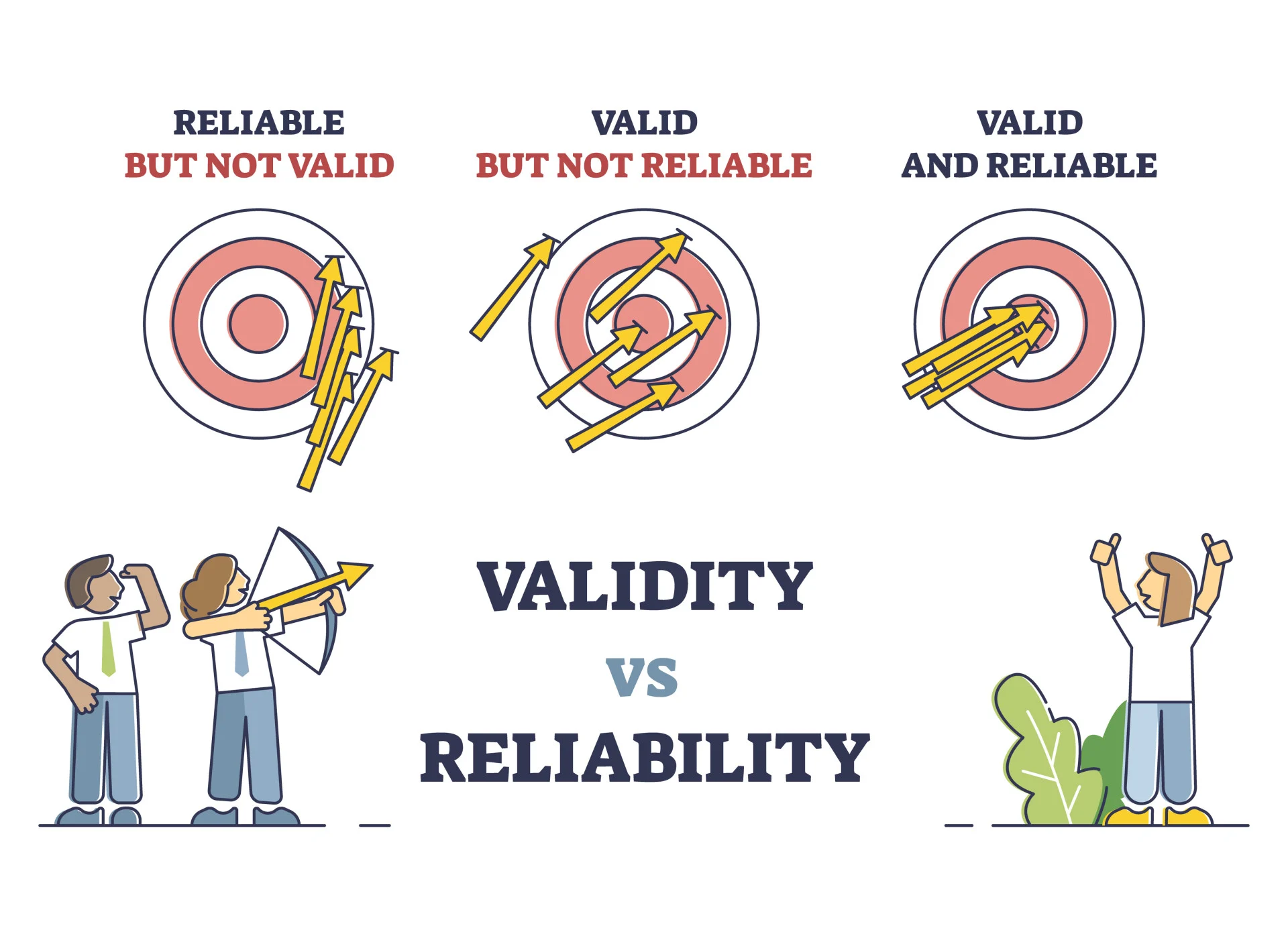
~~~~~~~~~~~~~~~~~~Validity VS Reliability~~~~~~~~~~~~~~~~~~~~~~~~~~~~~~
Validity:
Whether an instrument actually measures what it is set out to measure
Reliability:
Whether an instrument can be interpreted consistently across situations (is the instrument able to produce the same results under the same conditions consistently)
~~~~~~~~~~~~~~~~~~Systematic VS Unsystematic Variation~~~~~~~~~~~~~~~~~~
Systematic Variation
differences in the outcome created by a specific experimental manipulation (i.e., is the variation in the experiment is due to the experimenter doing something to one condition but not the others)
Unsystematic Variation
the variation that is not due to the effect in which we are interested in (i.e., the variation that results from random factors that exist outside of the experimental conditions - like confounding variables)
~~~~~~~~~~~~~~~~~~Central Tendency~~~~~~~~~~~~~~~~~~~~~~~~~~~~~~~~~
Mean: The average of a set of numbers, calculated by adding all the numbers together and dividing by the total count of numbers. It can be affected by extreme values (outliers). Best with interval or ratio data, but can be heavily affected by outliers
Median: The middle value in a sorted list of numbers. If there is an even number of observations, the median is the average of the two middle numbers. It is less affected by outliers compared to the mean.
Mode: The value that appears most frequently in a set of data. There can be more than one mode in a dataset if multiple values. Pros are it can be applied to any type of data and is not affected by outliers. a con is that we can’t do much with it
if there are two modes, it is bimodal
if there are more than 2 modes, it is multimodal.
~~~~~~~~~~~~~~~~~~Sample Statistics VS Parameters~~~~~~~~~~~~~~~~~~~~~~
Parameters
the value of a population is called a parameter. it is an estimate based on sampling data
Sample statistics
The value of a sample is called a statistic. This is because statistics are computed directly from actual data and are not estimates like parameters are.
~~~~~~~~~~~~~~~~~~Discrete VS Continuous Variables~~~~~~~~~~~~~~~~~~~~~
Discrete Variables: These are countable values that can take only specific values. For example, the number of students in a classroom can only be whole numbers (i.e., 1, 2, 3, etc.), and cannot be fractions or decimals.
Continuous Variables: These can take any value within a given range and can include fractional or decimal values. An example would be the height of individuals, which can be measured with great precision (e.g., 172.5 cm).
Week 2 Content:
~~~~~~~~~~~~~~~~~~~~Descriptive Statistics~~~~~~~~~~~~~~~~~~~~~~~~~~~~
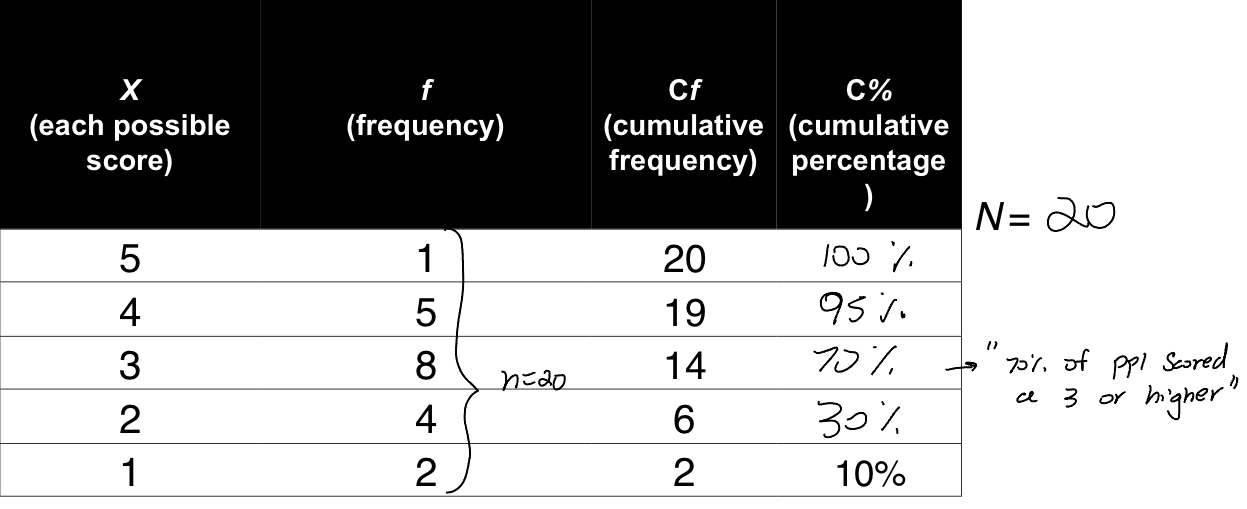
Frequency Distribution
a way of organizing data by the number of individuals located within each category of measurement
Frequency Distribution Percentages:
Converting the frequency into a percentage by doing F/N times 100
Cumulative Frequency
the number of people at or below that score
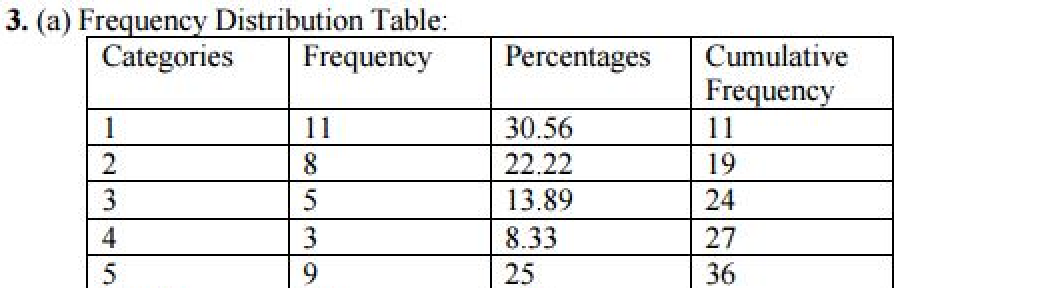
Percentile Ranks
percentile ranks are the % of people that are at or below that score
~~~~~~~~~~~~~~~~~~~~Frequency Distribution: Graphs~~~~~~~~~~~~~~~~~~~~~
Bar Graphs:
used with categorical variables (usually NOMINAL variables)
Histograms:
has a bar that represents each score, with the height of the bar representing the frequency of that score. (uses INTERVAL and RATIO variables)
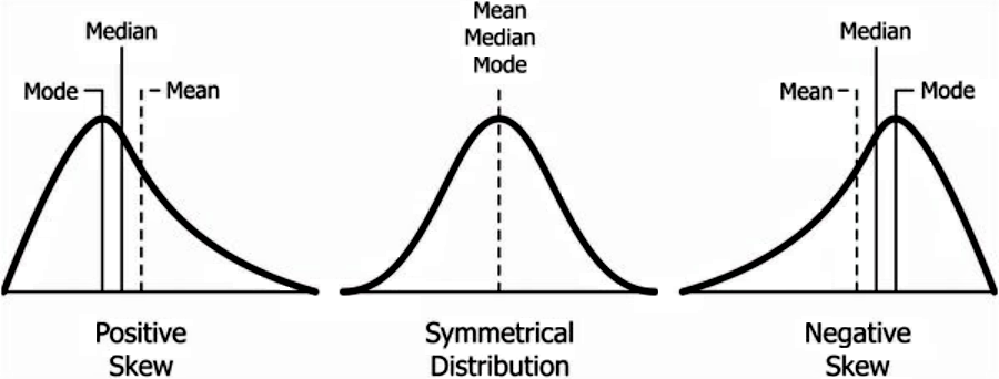
~~~~~~~~~~~~~~~~~~~~Shape of Distribution~~~~~~~~~~~~~~~~~~~~~~~~~~~~
with no skew, the mean, median, and mode are all the same. with skew, this changes.
(you can remember this by the tail of the positive skew pointing to the positive numbers, and the inverse for the negative)
Kurtosis: this term refers to the heaviness of the “tails”
Leptokurtic = heavy tails with a higher point
platykurtic = light tails and flatter
(you can remember that a platypus is low and flat to the ground)
graphs with a small standard deviation (closer to the mean) will look more platykurtic. graphs with a large standard deviation will be more leptokurtic.
Week 3 Content:
~~~~~~~~~~~~~~~~~~~~Sampling From Population~~~~~~~~~~~~~~~~~~~~~~~~~
When sampling from the population, it is important to randomly sample with high enough numbers
this is to avoid false positives or negatives. ultimately we want the sample to be representative of the population and this help to do so
when small samples are taken, we only get a small picture of the larger population.
~~~~~~~~~~~~~~~~~~~~Measuring the Fit of the Model~~~~~~~~~~~~~~~~~~~~~
The mean can be a problematic measurement of a sample because it is sensitive to extreme values or outliers. If there are outliers in the data, they can skew the mean, making it unrepresentative of the overall sample.
Additionally, in distributions that are not symmetrical (such as skewed distributions), the mean may not accurately reflect the central tendency of the data compared to the median or mode.
~~~~~~~~~~~~~~~~~~~~Variability~~~~~~~~~~~~~~~~~~~~~~~~~~~~~~~~~~~~
Variability:
the measure of how different the scores in your distribution are
reveals how similar (shown by a cluster) or different (shown by a large spread) your scores are
deviations
deviations of scores can be calculated by taking each score and subtracting the mean from it (i.e. if the mean is 5, and you scored a 2.6, the deviation is -2.4. if you scored a 7.3 when the mean is 5, the deviation is +2.3)
Adding deviations in order to find the “total error” won’t work because the numbers will be canceled. due to this, you need to find the sum of squares

Sum of Squares
in order to find the sum of squares, you square each deviation and add these new sums up.
Variance
variance is when you take the value found by the sum of squares and divide it by the number of scores inputted MINUS ONE. (so if your total sum of squares equated to 5.20, and you had 5 responses that created that sum of squares, your variance is 5.2/4 = 1.3) —> that 5 answers becomes 4 due to the -1 in the equation. the (n-1) is done in the equation to help account for sampling bias
BUT! there is a problem with variance. it is measured in “units squared”. this isn’t a very meaningful metric. SO, we take the square root of the variance (which is SS/n-1) and get the standard deviation
Standard Deviation
this is the most common measurement of variability. it deals with how far each score differs from the mean
“deviation” is the difference in scores from the mean
√(SS/n-1)
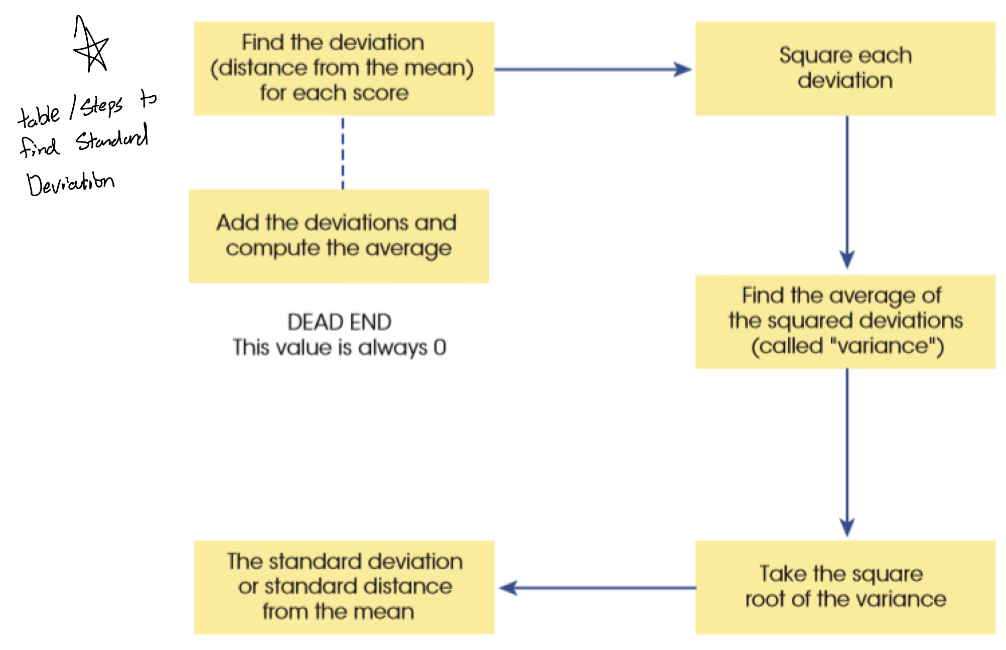
(Remember! the sum of squares, variance, and standard deviation all represent the same thing. the “fit of the mean to the data, the variability in the data, how well the mean represents the observed data and the error)
~~~~~~~~~~~~~~~~~~~~Standard Error (SE)~~~~~~~~~~~~~~~~~~~~~~~~~~~~~
Standard Error
the standard deviation of a sampling distribution
standard error = SD of the sample / √n
n = the sample size
standard error tells us how different the population mean will likely be from our sample mean.
Week 4 Content
~~~~~~~~~~~~~~~~~~~~Comparing Scores~~~~~~~~~~~~~~~~~~~~~~~~~~~~~~
Z-Scores:
Z-scores measure the number of standard deviations a data point is from the mean of a dataset. They are used to compare scores across different distributions or datasets, allowing for standardization regardless of the original scale of the data. A z-score can indicate how unusual or typical a score is in relation to the mean; for example, a z-score of 0 indicates the score is exactly at the mean, while a z-score of +2 indicates the score is two standard deviations above the mean.
A z-score can give insight into how well or meaningful a score is. If you got a 70% on a test, with a z-score of 0.8, and in another course, someone gets a 70% on their test with a z-score of 0.4, we know that the 70% with a z-score of 0.8 is more meaningful because it is further away from the norm (meaning you did better than others in the class)
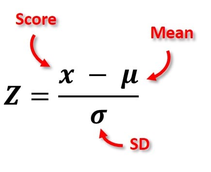
note: positive z-scores are above the mean, and negative z-scores are below the mean
standardization:
comparing with z-scores as they are one common unit (standard deviations) and can compare measures that are on different scales
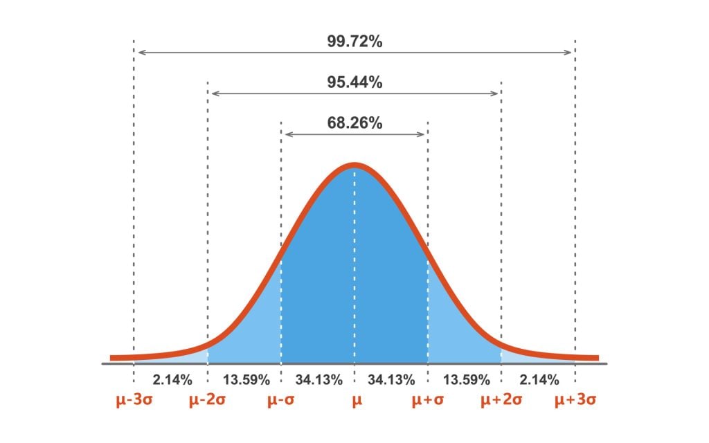
z-scores within a normal distribution
+1.96 and -1.96 are our magic numbers, as this spans the range that 95% of answers fall between (aka plus or minus 1.96 standard deviations in each direction)
~~~~~~~~~~~~~~~~~~~~Central Limit Theorem~~~~~~~~~~~~~~~~~~~~~~~~~~~
Central Limit Theorem
The Central Limit Theorem (CLT) states that the distribution of the sample means will approximate a normal distribution as the sample size increases, regardless of the original population's distribution. This is particularly useful because it implies that with a sufficiently large sample size, the sampling distribution of the mean will be normally distributed, allowing for the use of normal probability techniques even when dealing with non-normally distributed populations
(basically as the sample gets larger, the mean will get more normally distributed)
~~~~~~~~~~~~~~~~~~~~Confidence Intervals~~~~~~~~~~~~~~~~~~~~~~~~~~~~
Confidence intervals
if we know that 95% of scores fall within -1.96 and +1.96, we can use these values to calculate a confidence interval
confidence intervals are setting an upper and lower value that has the mean as the midpoint. This allows some wiggle room, and we can expect 95% of samples to have the true value of the population within the parameters.
WHAT CONFIDENCE INTERVALS ARE (AND ARE NOT)
the probability that the CI we generated includes the population is 95%
if you sampled 100 times, 95 of those samples would contain the true parameter
uncertainty range of an unknown parameter
It is NOT 95% confidence that the true population is in the interval
to find confidence intervals:
mean + or - (1.96* SE)
if the mean in the sample was 45, and your standard error was 5, a 95% confidence interval would be:
45 - (1.96×5) = 35.2
45 + (1.96×5) = 54.8
CI = 35.2-54.8
~~~~~~~~~~~~~~~~~~~~Covariance~~~~~~~~~~~~~~~~~~~~~~~~~~~~~~~~~~~
Covariance:
whether changes in one variable are met with changes in another variable (if one variable deviates from the mean, does the other variable deviate in a similar way?)
to calculate covariance, you must:
calculate the deviation between the mean and each subject’s scores in the first variable (x)
calculate the deviation between the mean and each subject’s scores in the second variable (y)
multiply these deviation values together (this gets rid of the negative signs)
add these values
the covariance is the average of these combined deviations

Issue: the UNITS! having 4.25 (lets say miles) is one thing, but if we converted it to kilometres it would be 11, which looks far more correlated even though its the same. to fix this we STANDARDIZE!
to standardize, we divide this covariance by the standard deviations of both variables
example:
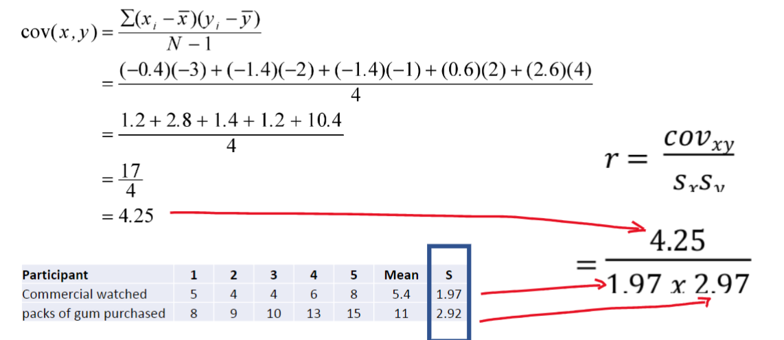
Correlation:
once this covariance is standardized, we now have a correlation!
correlation values fall between -1 and +1. 0 would = no relationship. -1 would be a perfectly correlated negative relationship, and +1 would be a perfectly correlated negative relationship.
(remember, though, correlation does NOT equal causation. there can be a third-variable in play that we are not examining.)
the correlation is r not r²
~~~~~~~~~~~~~~~~~~~~Spearman’s Rho Vs Kendall’s Tau~~~~~~~~~~~~~~~~~~~~
Kendall’s Tau:
The preferred method in general
better than Spearman’s for small samples with many tied ranks
Spearman’s Rho:
Pearson correlation on the ranked data. Only required ordinal data.
Week 5 Content
~~~~~~~~~~~~~~~~~~~~Ways To Describe A Straight Line ~~~~~~~~~~~~~~~~~~~
m
the “m” is the slope of the line. it gives insight to the direction/strength of the relationship
x
the “x” is the intercept of the line (value of Y when X=0)
Bᵢ
the “Bᵢ” is the regression coefficient for the predictor. it gives insight into the slope of the regression which shows the direction and strength of the relationship
B₀
The “B₀” is the intercept (value of Y when X=0) aka, when the predictor variable is equal to zero
~~~~~~~~~~~~~~~~~~~~Regression~~~~~~~~~~~~~~~~~~~~~~~~~~~~~~~~~~~
Regression:
regression is a way of predicting the value of one variable from another.
its a slightly fancier version of a Pearson Correlation
~~~~~~~~~~~~~~~~~~~~Method Of Least Squares~~~~~~~~~~~~~~~~~~~~~~~~~
Method of Least Squares
creating a line of best fit that summarizes the data in a way that reduces the error (if a line of best fit is off, it will have more error)
~~~~~~~~~~~~~~~~~~~~Sum of Squares Model~~~~~~~~~~~~~~~~~~~~~~~~~~~
SS Model
one reason we use regression and not mean is because the mean is static, so no matter what your predictor or X variable is set to, the Y will remain static. we can use the SS model to calculate the sum of squares and show how much better the regression model is than the mean (SSm = sum of squares of the mean)
if the SSm is large, then the linear model has made a big improvement to how well the outcome variable can be predicted
if the SSm is small, then using the linear model is considered only a little better than using the mean. (i.e. the regression model is only slightly a better fit than the mean)
I believe you’d want the SSm to be high because of this
The sum of squares in regression analysis is divided into three components:
Sum of Squares Total (SST): This represents the total variability in the dependent variable. It is the sum of the squared differences between each observed value and the overall mean of the dependent variable. It measures how much the data varies overall.

Sum of Squares Model (SSM): This reflects the variability explained by the regression model. It is the sum of the squared differences between the predicted values from the regression model and the overall mean of the dependent variable. A larger SSM indicates that the regression model provides a better fit and explains more variability in the data.

Sum of Squares Residual (SSR): This measures the variability not explained by the regression model. It is the sum of the squared differences between the observed values and the predicted values from the model. A smaller SSR indicates that the model is better at predicting the observed values.

~~~~~~~~~~~~~~~~~~~~F-Value~~~~~~~~~~~~~~~~~~~~~~~~~~~~~~~~~~~~~~
F-value
F is calculated using the average sums of squares (referred to as the mean squares or MS)
F= MSm/MSr (I belive MSm is the mean squares of the model and MSr is the mean squares of the residuals)
I think you want the MSm to be a higher number and the MSr to be a lower number.
A residual is how far away a point is vertically from the regression line. Simply, it is the error between a predicted value and the observed actual value
~~~~~~~~~~~~~~~~~~~~R² Value~~~~~~~~~~~~~~~~~~~~~~~~~~~~~~~~~~~~~
R²
this is different than correlation but somewhat similar. it shows the proportion of variance between two variables accounted for by the regression model
If R² is 0.43, then you could say 43% of the variation in the dependent variable is caused by the predictor variable/independent variable
~~~~~~~~~~~~~~~~~~~~Null Hypothesis Significance Testing~~~~~~~~~~~~~~~~~
NHST
The Null Hypothesis states that there is no relationship. If you failed to reject the null hypothesis, you’d be saying there is no relationship (reject if p=<0.05)
the Alternative Hypothesis states that there is a relationship between the predictor variable and the outcome variable. if you reject the null hypothesis theory, you’d be saying that you’re accepting the alternative hypothesis, and as a result, saying there is a relationship between the predictor and outcome variables.
by DEFAULT we should assume the null hypothesis to be TRUE. only after we get a p value of <0.05 can we reject the null (cuz it would mean that only <5% of the time that result should occur if no relationship exists between the variables)
the most common alpha value in NHST is 0.05 or 5%
Type 1 NHST Errors
Type one errors are when you reject the null hypothesis theory when it was actually true (meaning you said there was a correlation when there wasn’t). basically you sounded a “false alarm”.
Type 2 NHST error
type two errors are when you fail to reject the null hypothesis theory that is actually false (meaning you said there as no correlation when there actually is). this typically happens when your effect was too small.