Interpretation of inferential statistics


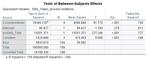
There are statistically significant differences in postDAQ levels between the conditions when adjusted for baseline DAQ, there is a difference between at least two of the groups (potentially more) but it does not tell us which specific groups are significantly different from each other. We require a post-hoc test
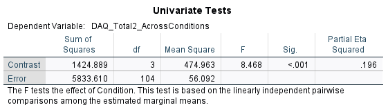
The Partial Eta Squared value indicates the effect size for the conditions is small ( ηp2 = 0.196).
F (3, 104) = 8.47, p < .001, ηp2, = .196
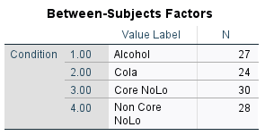
A one-way ANCOVA with drink cue type as the independent variable, (divided into four levels/ conditions: advertisements of Core NoLo drinks, non-core NoLo drinks, alcoholic drinks or soft drinks), post DAQ scores as the dependent variable and baseline DAQ scores as a covariate was conducted.
The results showed that there was a significant effect of post DAQ scores in different advertisement conditions when accounting for baseline DAQ scores (F (3, 104) = 8.47, p < .001, ηp2, = .20) with an effect size that indicated 20% of the total variance was attributable to drink cue types.
Bonferroni-adjusted pairwise comparisons revealed that post DAQ scores were significantly higher in the alcohol condition than in the cola condition (MD = 10.30, p < .001), Core NoLo condition (MD = 7.00, p = .004) and Non Core NoLo (MD = 6.16, p = .018). Though each difference of post DAQ scores between the cola condition, core NoLo condition and non core NoLo condition were found not statistically significant, the smallest difference observed was between the core NoLo condition and non core NoLo condition (MD = .842, p = 1.000).
There is a 10.30% difference between the mean post DAQ scores of alcohol and cola conditions, this is significant.
There is a 7.00% difference between the mean post DAQ scores of alcohol and core NoLo conditions, this is significant.
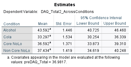
Comparing the estimated marginal means showed that the highest post DAQ scores were observed in the alcohol condition (M = 43.59) compared to cola (M = 33.30), core NoLo (M = 36.59) and non-core NoLo (37.43).

Compare the significance values, report these results in a similar manner to one-way ANOVA, but substitute ‘means’ for ‘adjusted means’
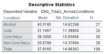
These provide the adjusted means following the inclusion of the covariate (where as the original descriptive table shows means without covariate involved).
Alcohol-cola, p < .001 (significant)
alcohol-core NoLo, p = .004 (significant)
alcohol- non core NoLo, p = .018 (non-significant)
cola-core NoLo, p = .680 (non-significant)
cola- non core NoLo, p = .298 (non-significant)
Core NoLo- non core NoLo, p = 1.00 (non significant)
to be significant the p < .016

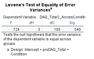
Using homogeneity tests ticked off during ANCOVA- are we supposed to have levene’s tests in our inferential outputs?
When reporting things in the inferential statistics, if we supply the information in a table or in the appendix do we still have to write out all of the means or do I do what I did for the descriptive statistics?
when reported the means from the estimated marginal means section, why do I report the SE and do I report this in the same bracket as the m such as (M = , SE = _)?
When you said to add a column of the statistics in my descriptives table, like the ANOVAs and chi square is it the total column of each varibale then instead of adding each one for each condition?
Estimated Marginal Means
conditions

From the adjusted means, participants in the alcohol condition had the highest postDAQ scores on average adjusting for baseline DAQ scores (M = 43.59) whilst the lowest postDAQ scores were on average reported in the cola (M = 33.30) (see appendix _).
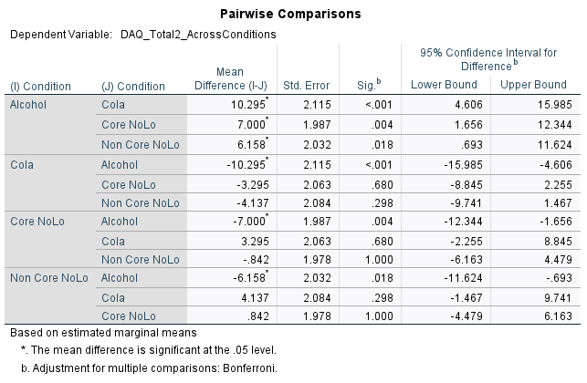
There is a significant difference between the alcohol condition and cola condition (p < .001). There is a significant difference between the alcohol condition and Core NoLo condition (p = .004). There is a significant difference between the alcohol condition and the non-core NoLo condition (p = .018). There are no significant differences between any of the other conditions.