Financial Econometrics
CAPM
FAMA-FRENCH MODEL
Problem: CAPM alone doesn’t explain all asset returns.
Solution: Fama and French propose two additional factors:
SMB (Small Minus Big): Return difference between small- and large-cap stocks.
HML (High Minus Low): Return difference between high and low book-to-market stocks.
Model equation (for each asset i at time t):
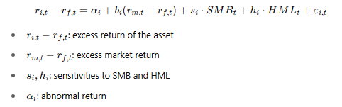
Fama-French 3-factor model is better than CAPM, based on R².
However, two important limitations:
Instability of parameters over time.
Non-zero alphas imply incomplete explanation of returns—even with 3 factors.
Risk Analysis
BOOTSTRAP
Problem: Asymptotic results (like normal distribution of estimators) are only reliable with large samples
With small samples, these approximations can be misleading → confidence intervals (CIs) may be too narrow or too wide
Solution: Use bootstrap if dataset = small to simulate a large number of samples & better approximate the sampling distribution
Bootstrap CI Procedure
Estimate the parameter θ from original sample
Create B (large) random samples (with replacement) of the same size (T) from the original data with replacement
Compute θᵇ (estimate) for each sample.
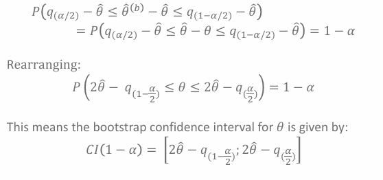
Use the quantiles of the empirical distribution of θᵇ − θ to form a confidence interval

Key Point:
Even if we don’t know the exact distribution of θᵇ, we can estimate percentiles (quantiles) from the bootstrap distribution.
In addition, we can argue that we can estimate the distribution of

This makes sense if we assume that 𝜃_hat arises from sampling from a distribution with parameter 𝜃 & 𝜃^b_hat from 𝜃_hat
→ Bootstrap procedure only works with independent data
If a dependency → Block bootstrap
Block Bootstrap solves dependency issue:
Instead of resampling single observations, resample blocks of consecutive data points.
Divide data into k blocks of size l (where ).
Rule of thumb:
Preserves local dependency.
Still consistent, but slower convergence than regular bootstrap.
BUT
Block bootstrap intervals are wider → means usually not as accurate as the traditional bootstrap
Block bootstrap allows to deal with a degree of dependency between observations not possible with the traditional bootstrap
TESTING STATIONARITY
2 types of stationarity
Strong (strict) stationarity:
Joint distribution of observations does not change over time. That is, when the distribution (Yₜ₁, ..., Yₜₙ) has the same distribution as (Yₜ₁₊ₕ, ..., Yₜₙ₊ₕ) for any h
Weak stationarity: The series has:
Constant mean
Constant variance
Covariance independent of t
→ In econometrics, we usually test weak stationarity
Rule of Thumb to detect (non-)stationarity
Visual check: Plot the time series:
If path oscillates around the mean often → likely stationary
If there's a trend or the mean shifts → likely non-stationary
Non-stationarity test - Dickey-Fuller
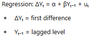
→ unit root = non-stationary
→ stationary
! NOT use standard t-test, because under the process is not stationary !
→ Critical values have been tabulated (Fuller 1976)
Testing Procedure
Tests with H₀ = non-stationary:
Dickey-Fuller ; Augmented Dickey-Fuller (ADF) ; Schmidt-Phillips ; Elliott-Rothenberg-Stock
RH0 (p-value < ) : reject non-stationarity → stationary series
NRH0 (p-value > ): non-stationary fails → non-stationary series
Tests with H₀ = stationary:
KPSS test (Kwiatkowski et al.)
RH0 (p-value < ) : is not stationary → non-stationary
NRH0 (p-value > ): cannot say is stationary → stationary
Models that require stationarity:
most time series models
ARMA, ARCH, GARCH → ACF & PACF
Linear regression models on time series (OLS)
Bootstrap (if not stationarity → Block bootstrap)
VaR, ES
ARMA, ACF & PACF
Wold Theorem → building block of the ARMA process
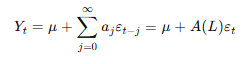
Main idea: Any stationary time series can be written as a linear function of current and past white noise .
Lag operator
Key formula:
ARMA Process
Instead of infinite terms, approximate with finite polynomials:
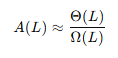
Leading to:
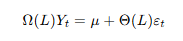
General ARMA(p,q) form:
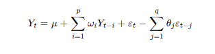
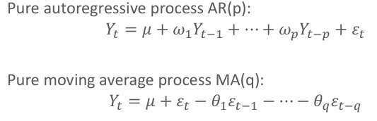
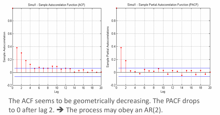
AR(p): regressed on past values → PACF cuts off after lag p
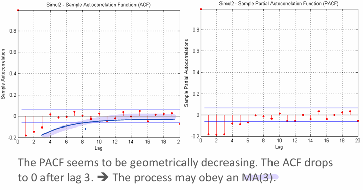
MA(q): regressed on past shocks → ACF cuts off after lag q
ACF & PACF
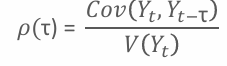
ACF: Measures correlation between and
PACF: Measures correlation of & after removing intermediate lags
In an model: PACF = coefficient on lag
→ identification of p & q with ACF & PACF
Residuals analysis
After fitting a model, residuals should be white noise (stationarity)
Use Ljung-Box or Box-Pierce test:
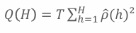
→ Q(H) should be close to 0, IF residuals = white noise
ARMA Procedure
Check stationarity (Dickey-Fuller test)
Identify p & q from ACF (for MA) / PACF (for AR)
Estimate ARMA(p,q) model
Check residuals for white noise (Ljung-Box test)
RH0 (p-value < ) : reject significant autocorrelation exists → model = inadequate
NRH0 (p-value > ): no significant autocorrelation & residuals are white noise → model = well specified
Key rules
AR(p) → ACF tails off gradually
MA(q) → ACF cuts off sharply after q
ARCH & GARCH
AR models, variance (volatility) is assumed constant over time (homoscedasticity)
Reality: Financial series often show volatility clustering (periods of high/low volatility)
Solution: Model volatility to depend on past → ARCH model (Autoregressive Conditional Heteroscedasticity)
BUT when estimated on financial data, ARCH(p) usually needs large number of p of significant lags
Solution: GARCH (Generalized ARCH) model
2 - Step Procedure (ARMA(p1, q1) - GARCH(p2, q2))
Step 1 (mean)
Use ACF/PACF plots to select p1 & q1
Estimate ARMA(p1,q1) model
Check residuals for white noise (Ljung-Box test + ACF/PACF of residuals)
RH0 (p-value < ) : Residuals ≠ white noise, this means model missed some autocorrelation → model ≠ adequate
NRH0 (p-value > ): Residuals = white noise, this means model captured the mean structure well → model = fits well
Step 2 (variance)
Test for ARCH effects
ACF/PACF of squared residuals
Formal ARCH test: Regress on its lags, compute , compare to chi-squared
RH0 (p-value < ) : Significant evidence of ARCH effects, this means the residuals show some time-varying volatility → GARCH model = needed
NRH0 (p-value > ): No evidence of heteroskedasticity (volatility clustering), this means the model has constant variance → no need for GARCH
Use ACF/PACF of squared residuals to select p2 & q2
Estimate GARCH(p2,q2) model
Check residuals after GARCH for remaining ARCH effects (compute ARCH test + ACF/PACF of ARMA(p1,q1) - GARCH(p2,q2) squared residuals)
ARMA-GARCH model
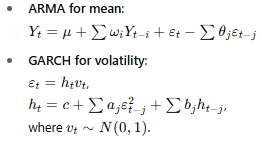
→ GARCH(p2, q2) can be rewritten as an ARMA model on squared Y’s errors (not directly on squared observations):
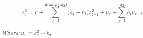
This form shows how past squared errors and volatility affect current squared error