Quantitative Statistics - BSNS 112 - Lecture Notes
Topic 1 - Probability - Chapter 6 - Slide Set 1
Required: Read Chapter 6.1 and 6.2.
The rest is extra reading.
Watch the YouTube tutorial on how to use excel.
Most important information is between 20-37 minutes.
How to drag a formula down (to get “taxable income”)
How to do this with an absolute reference (to get “taxes to be paid”)
Conditional probabilities tell you how you should rationally update your beliefs in response to evidence. E.g.
Real world example: If you learn that the price of shares on the US stock market has fallen, how should you change your assessment of the likelihood that the price of shares on the NZ stock market will fall?
Random Experiments
A random experiment is a process or action where the outcome is uncertain, and cannot be predicted with certainty beforehand. No 2 outcomes can occur at the same time (they are “mutually exclusive”).
There are 2 conditions that the outcomes must satisfy in a random experiment:
Each outcome must have a probability between 0 and 1.
The probabilities of the outcomes must sum to 1.
A simple example of a random experiment would be rolling a standard die. We assume that this die is fair. The sample space for the experiment would be:
S = {1,2,3,4,5,6}
The probability (P) of each outcome is 1/6.
Sample space (S): the set of possible outcomes. Must include all possible outcomes (list is “exhaustive”).
Fair = Unbiased.
Probability = P.
Events
Event (E): Any subset of a set of outcomes.
E.g. (for dice):
What is the probability of the event that the outcome is odd? Eodd = {1,3,5}
What is the probability of the event that the outcome is small? (We will define small as a number less than 3). Esmall = {1,2}
The probability of an event is the sum of the probability’s of the outcomes in the event. E.g.
P(Eodd) = P(1)+P(3)+P(5) = 1/6 + 1/6 + 1/6 = 3/6 = 1/2
If the probability of each outcome is the same, then you can use the formula:
P(E) = No. of outcomes in E ÷ No. of outcomes in S
Venn Diagrams
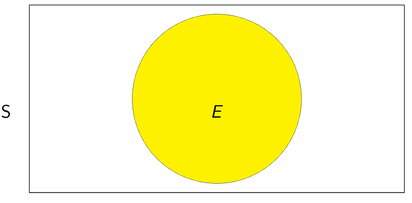
Venn Diagrams show our sample space values and are used to represent interactions between different events.
As an event (E) is a subset of S, we can represent it as an area contained in the rectangle representing S.
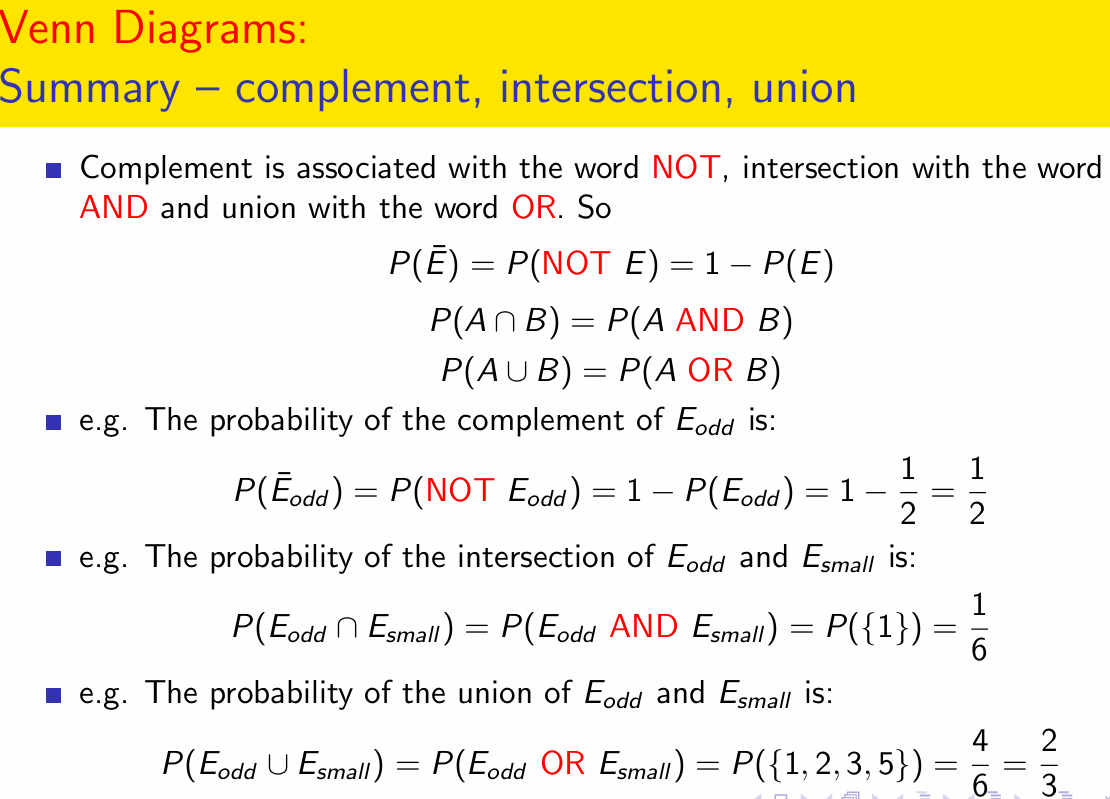
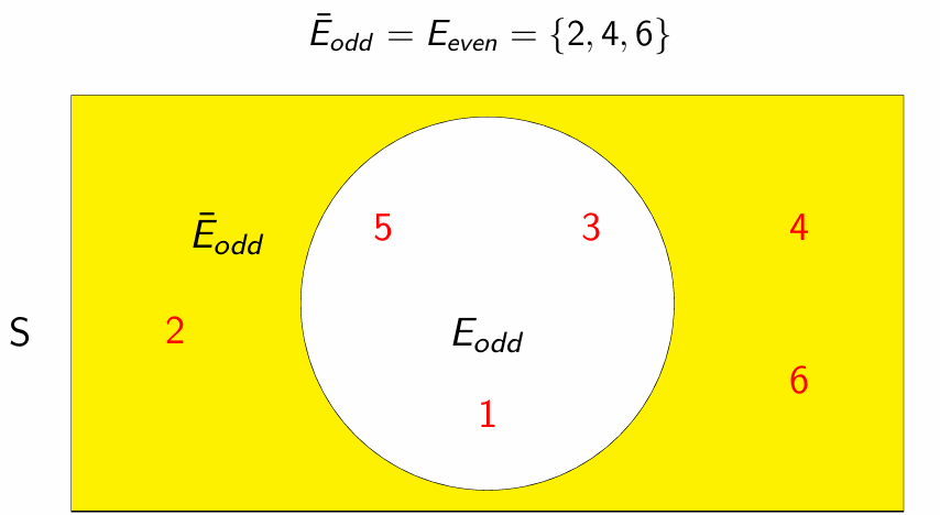
Complement: NOT Symbol: Ē Probability is: P that E does not happen.
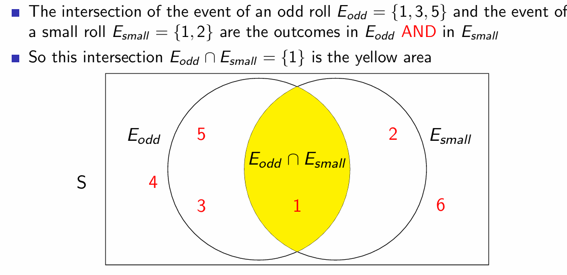
Intersection: AND Symbol: ∩ Probability is: P of A+B
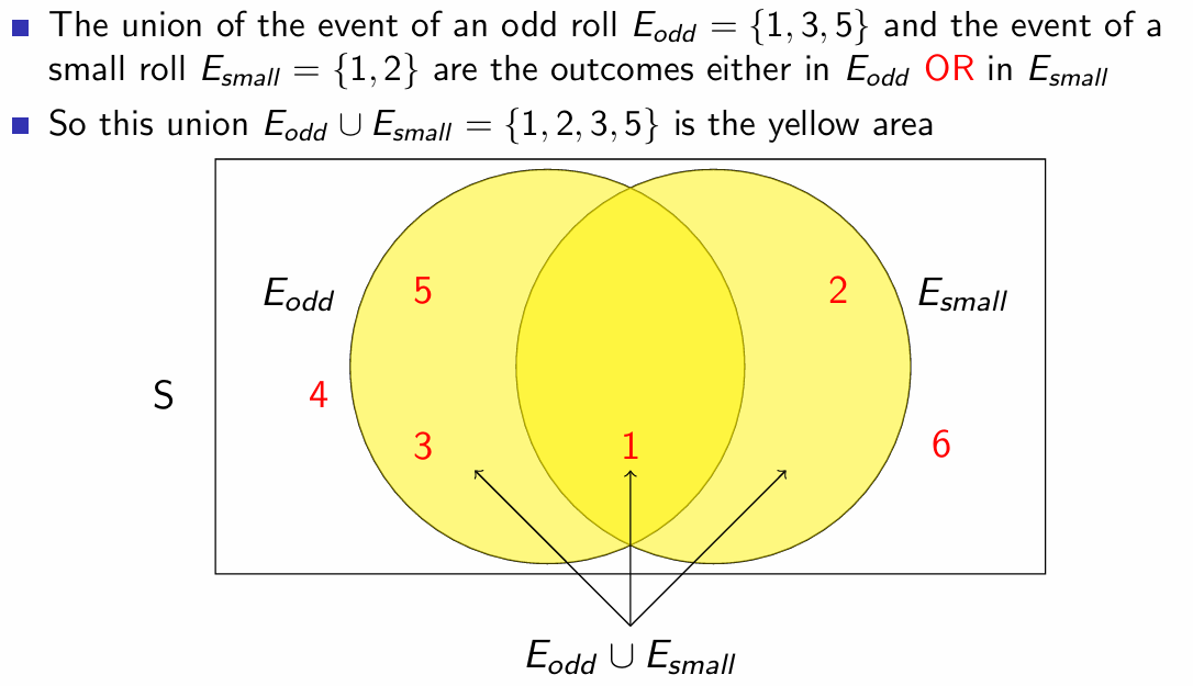
Union: OR Symbol: ∪ Probability is: P = A or B
These words (NOT, AND, OR) are crucial words. They are called “logical connectives”.
In context:
Suppose you are designing a survey for the government. Your random experiment involves choosing NZ adults at random from the population. Your boss asks you about the probability of this event: Either they are male OR they both have a high income AND they are NOT from Auckland.
You can analyse this event as follows, and draw a Venn Diagram:
[male] ∪ [high income ∩ Auckland]
Complement (Ē)
The complement of an event (E) is the outcomes in S that are not included in the event. The symbol for this is Ē. We can represent it in the rectangle (sample space) as the area in S that is NOT in E.
The dice example:
Intersection (∩)
Intersection means any outcomes that cross over between 2 separate events.
The dice example:
Union (∪)
A union is when 2 or more events are combined to form a new set. In includes everything that occurs in both events. The “OR” just means it includes outcomes that happen in either set (inclusive of all events).
The dice example:
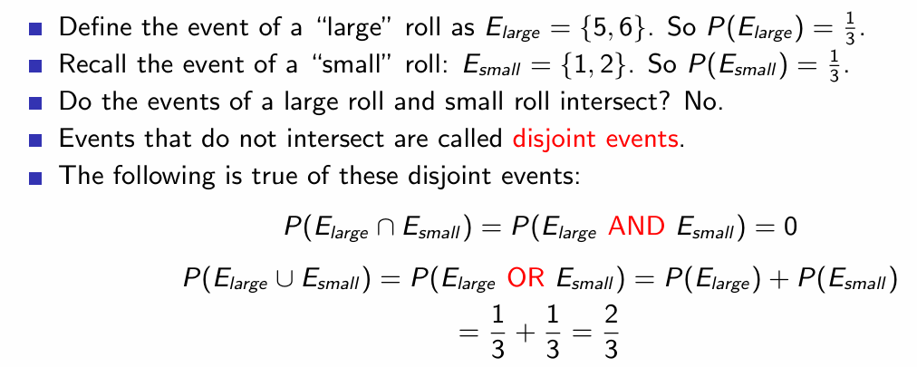
Disjoint Events
Disjoint events are events that do not intersect.
In general, when considering any 2 disjoint events, A and B. The:
Probability of their intersection is 0:
P(A∩B) = P(A AND B) = 0
Probability of their union is the sum of their probabilities:
P(A∪B) = P(A OR B) = P(A) + P(B)
The dice example:
Types of Probabilities
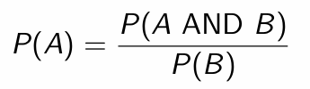
Joint Probability
Joint probability is the probability (P) of 2 events (E) both happening. (The P of the intersection of the 2 events).
Example:
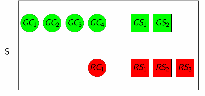
What is joint probability a draw is green AND a circle? P = 4/10
What is joint probability a draw is red AND a square? P = 3/10
Marginal Probability
Marginal Probability is just the probability (P) of 1 single event occurring.
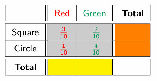
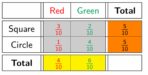
Table of Joint and Marginal probabilities:
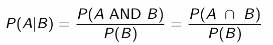
Conditional Probability
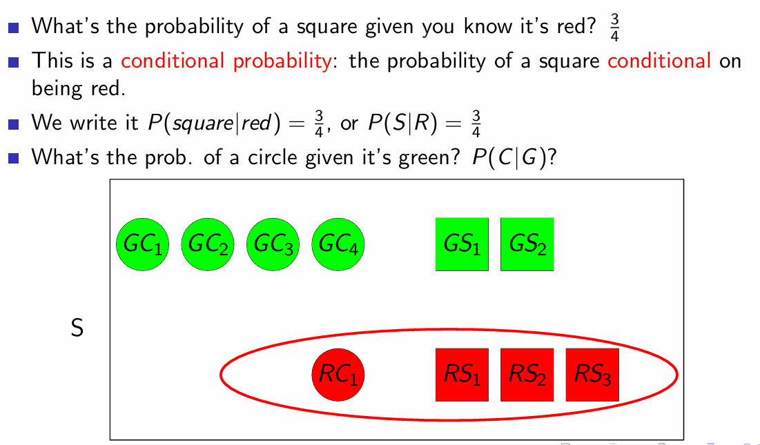
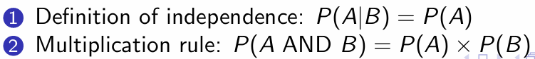
Generally we write it as P(A|B) (where A is the event, and B is the condition).
The general formula for P of A conditional on B:
Independence
Independent means that your assessment of Probability for A does not change when we learn that B (a condition) has occurred.
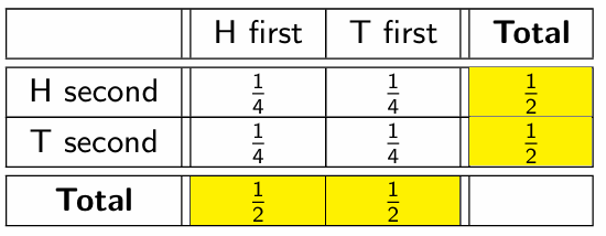
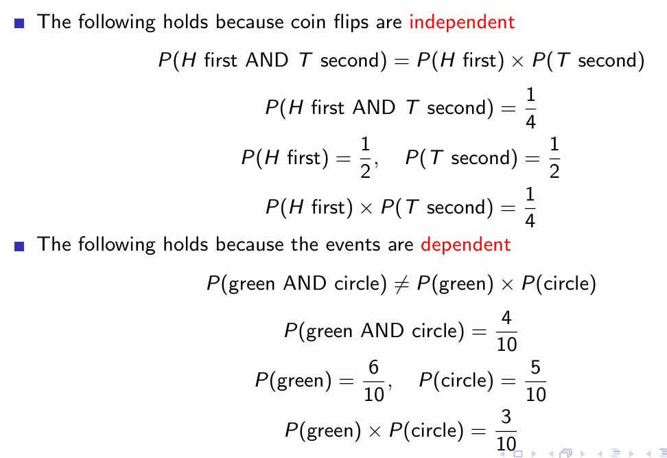
Random Experiment 3: Flip a fair coin twice in a row.
S = {HH, HT, TH, TT}
If we learn that Tails was the second flip, do we change our assesment of the probability of heads being first?
No, it does not matter what the second event is as heads will still be ½ either way, therefore the events are independant.
Events are independent if:
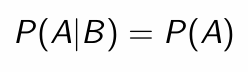
OR
Dependence
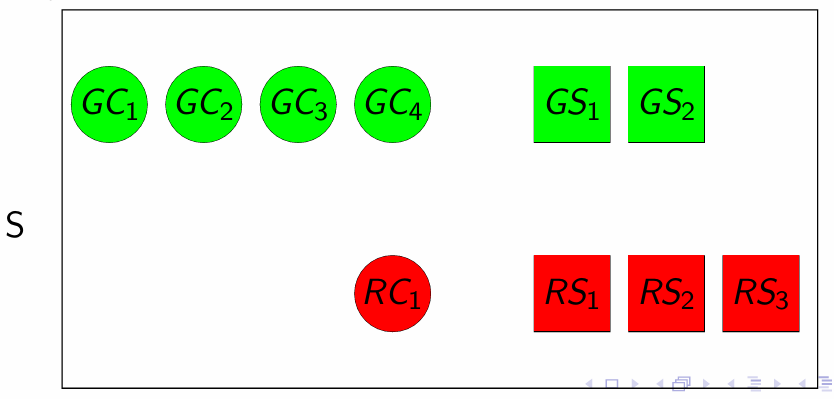
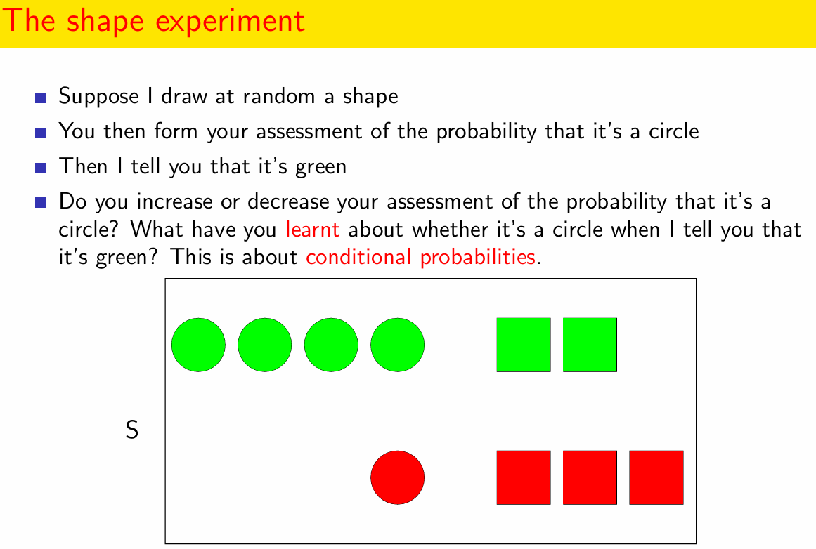
Suppose someone draws a random shape from this box. I asses the probability that it is a circle P(C) = ½
Then I am told that the shape is green. I then reassess my probability of it being a circle to P(C|G) = 2/3
Because I changed my assessment after learning a condition the event is dependant, i.e. the event depends on the condition.
As P(C|G) =/ P(C), the event of being green and being a circle are dependant events.
Multiplication Rule
A way to determine whether events are independent or dependent.
Summary of Independence/Dependence
There are 2 methods for checking if events are independent.
Topic 2 - Discrete Random Variables - Chapter 7
Read Chapter 7.1, 7.2, 7.3, 7.4 and 7.5a-b.
The rest is extra reading.
Random Variables and PMF
Expected Value (E) and Variance
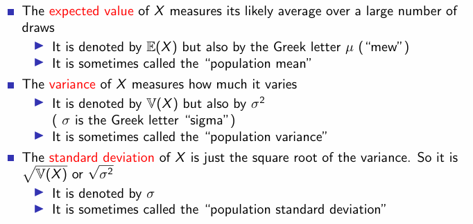
Expected Value
Variance
A high variance (higher number) means that the outcomes vary a lot.
It measure the amount that outcomes tend to vary from their expected value - it measures the risk.
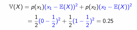
The Variance X (denoted V(X), is the probability weighted average of the square of the difference between the outcome and the expected value.
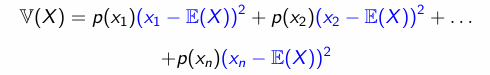
In use with unbiased coin flip example:
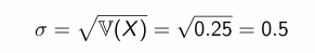
Standard Deviation
Standard deviation of X is the square root of the variance.
Another way of measuring risk. If Standard Deviation is high, so is variance.
Summary
Binomial Random Variable
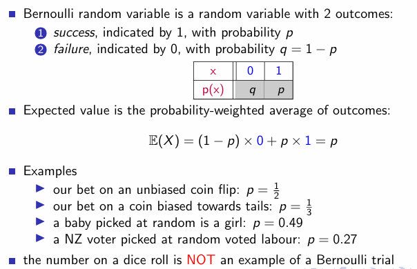
Bernoulli Random Variable
Take the notes after this (first 17 minutes of the lecture)
Cumulative Distribution
uhhh.
Bivariate Distribution
Shows joint probability for each pair of outcomes.
Is just a way to relabel our events with numbers, which changes out random experiment into a random variable. This is done to allow us to define expected values and variances that you could not before.
Correlation
Two random variables are positively correlated if they tend to “move in the same direction”.
When X is low, Y is low. When X is high, Y is high.
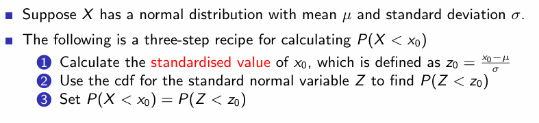
Topic 3 - Continuous Random Variables
pdf = Probability Density function
cdf = cumulative distribution function
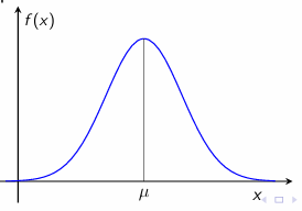
Normal Distribution
Intro to Normal Distribution
Height of a given demographic, will have (approximately) a normal distribution.
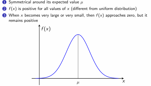
Bell shaped
we write its expected value as E(X) = μ (mu) which is also referred to as the “population mean”
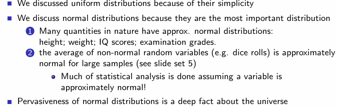
All things held equal, things will fall into a normal distribution
Normal distribution is symmetrical either side of mew
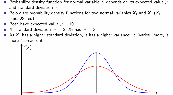
Higher standard deviation means it has higher variance (i.e. it varies more) and the curve is flatter
Standard normal distribution
Expected Value is 0
Standard Deviation is 1
Super godamn important, must remember Standard deviation is the square root of the variance
Example:
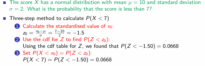
Calculating cdf probabilities
Calculating other probabilities
From probabilities to outcomes
Topic 4 - Sample Statistics
Measures of central tendency
Sample Median
The middle of the outcomes. duh
Mean can be higher than median when there are items in the sample with very high results.
Sample Mode
Most common number (duh)
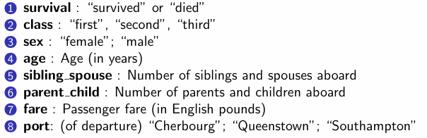
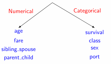
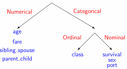
How to classify variables
Numerical vs Categorical
Numerical - value is inherently a number
Categorial Cariable - is a category (although can have a numerical value)
Titanic Example
Ordinal vs Nominal
ORdinal - of categorical, has a natural order
Nominal - any that are not ordinal
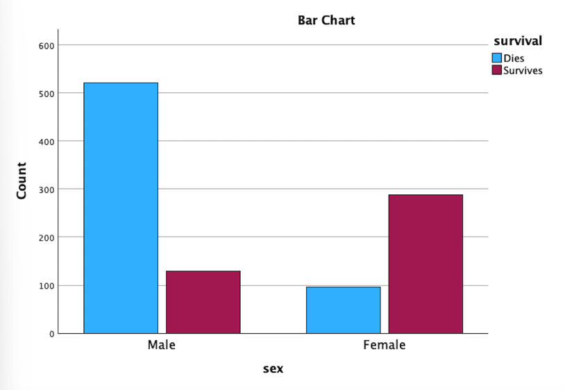
Frequency Bar chart
categorical variables such as sex and survival, the frequency of each category can be depicted by this chart
What can we conclude from this bar chartSample
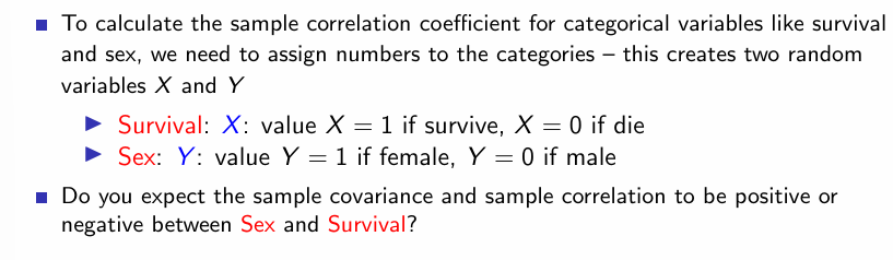
Covariane and Correlation
Topic 5 - Distribution of the Sample Mean
Distribution of the sample mean (X with line over it): Dice Example
Distribution of the sample mean (X with line over it): General case
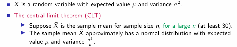
The central limit theorem (CLT)