Mechanotechnics N4 Complete Comprehensive Study Guide

Workshop Layout

• Definition & Concept: Workshop layout refers to the spatial plan or arrangement of machinery, equipment, work areas, storage facilities, material handling paths, and worker amenities on a factory or workshop floor.

• Symptoms of Poor Workshop Layout:

  • Inadequate management and operational control.

  • Long and indirect material transport routes.

  • Severe aisle congestion and frequent industrial accidents.

  • Production line bottlenecks causing extensive delays.

  • Unnecessary handling of raw materials and workpieces.

  • Subsubstantial decrease in overall worker performance and morale.

• Advantages of Good Workshop Layout:

  • Minimization of production costs and manufacturing time.

  • Production of higher-quality goods at faster throughput rates (efficient production).

  • Easier supervision, control, and monitoring of workshop personnel.

  • Enhanced job satisfaction and worker safety.

  • High adaptability to future changes in production systems or product lines.

• Ten Principles of Good Workshop Layout:

  • Flexibility (Adaptability): Easily reconfigured to accommodate new products or changing production volumes.

  • Co-ordinated Services: Good communication channels and close proximity between production departments, administrative offices, and main service points.

  • Accessible Service Points: Utility connection points (plugs, compressed air, water, gas) are easy to find and located close to machinery requiring planned maintenance.

  • Clear Transport Routes: Unobstructed aisles and transport pathways designed for safe movement.

  • Optimum Use of Space: Effective utilization of available floor space and vertical space while maintaining easy accessibility.

  • Minimum Travelling Distances: Shortest possible movement paths for both personnel and raw materials.

  • Minimum Material Handling: Reduction of workpiece handling to the absolute minimum necessary.

  • One-Way (Unidirectional) Flow: Unidirectional movement of materials and products through sequential operations to avoid backtracking.

  • Pleasant Working Conditions: Ample light, ventilation, noise reduction, and ergonomic arrangements.

  • Worker Safety and Equipment Security: Adherence to labor laws (such as the Basic Conditions of Employment Act) and physical safety precautions.

• Factors Influencing Layout Design:

  • Type of production (mass, batch, or individual).

  • Effective flow rates and required output volume.

  • Nature and complexity of inspection requirements.

  • Specific type and quantity of machinery and equipment needed.

  • Quantity, mass, and storage space requirements of raw materials, by-products, and waste.

  • Sequential operational flow of manufacturing processes.

  • Local council building regulations and environmental laws.

  • Availability and capacity of additional services (water, gas, compressed air, electricity).

  • Availability of suitably qualified and skilled labor.

  • Floor carrying capacity (weight limit per unit surface area).

• Types of Production Methods:

  • Mass Production:

  • Characteristics: Extremely large production quantities, short individual processing time, low unit labor costs, highly mechanized/computerized equipment, continuous mass flow, specialized single-purpose machinery, bulk storage requirements, and favorable break-even volume.

  • Batch Production:

  • Characteristics: Identical products produced in specific groups or lots; work divided into distinct operations; high specialization using process layouts; small-scale to medium-scale operations; multi-purpose machines; flexible and adaptable production methods; requires highly trained workers.

  • Individual Production:

  • Characteristics: Manufacturing one customized item or project at a time; requires versatile, highly skilled artisans; high capital expenditure ($\text{CAPEX}$); specialized custom tooling; flexible physical layout.

• Types of Workshop Layouts:

  • Process Layout (Functional Layout):

  • Machines of similar function or operating type are grouped together in dedicated sections (e.g., Lathe Section, Drilling Section, Milling Section, Grinding Section, Inspection Section).

  • 
    

  

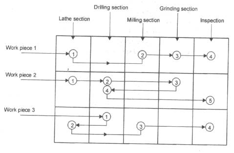
  • Requirements: Economical placement of sections, shortest possible transport paths between departments, highly skilled workforce, strict supervisory control, adaptable inspection procedures, carefully planned routing.

  • Advantages: Multi-purpose machinery utilization, flexible production lines, complete machine utilization, immunity to total system stoppage if one machine breaks down, low defective rejection rate.

  • Disadvantages: Non-continuous product flow, extensive material handling, high costs due to rigorous individual inspection, large floor space demands, complex scheduling and routing control.

  • Product Layout (Line Layout):

  • Machinery and equipment are arranged strictly in the physical order of the manufacturing sequence required to assemble a specific product.

  • Requirements: Sufficiently large production volume, minimal design changes, consistent raw material supply, plentiful spare parts, standardized inspection points, meticulously planned scheduling.

  • Advantages: Minimum material handling, short production cycles, simplified production control and supervision, effective use of unskilled labor, uninterrupted flow, continuous automated inspection.

  • Disadvantages: Extreme lack of operational flexibility, heavy reliance on costly specialized machinery, single machine breakdown halts the entire line, higher product rejection rates during line faults.

  • Fixed Position Layout:

  • The product remains stationary due to size or weight (e.g., aircraft, ships), and workers, tools, and machinery are brought to the site.

• Layout Procedures and Tools:

  • 2D Model Layout: Uses layout boards and scaled cardboard templates with color coding. Advantages include low cost, no specialized computer hardware needed, and ease of use by non-experts. Disadvantages include storage difficulties, inability to show vertical height, and fragility.

  • 3D Model Layout: Uses physical scale models. Highly accurate and excellent for visualizing complex multi-story plants, but extremely expensive and space-consuming.

  • Computer-Aided Design (CAD):

  • Advantages: Rapid drawing generation, easy modification of ideas, full 2D/3D visual modeling, accurate integrated engineering calculations, simple electronic storage, quick feasibility studies, dynamic layout adjustments.

  • Disadvantages: High cost of software/hardware, potential shortage of skilled draughtspersons.

Metal Protection and Corrosion

• Fundamentals of Corrosion:

  • Processed metals (such as carbon steel) exist in an unstable, high-energy state and naturally tend to revert to their stable, lower-energy chemical forms (such as iron oxide / rust) via chemical or electrochemical reactions with environmental moisture and oxygen.

• Classification of Corrosion:

  • Chemical Corrosion (Direct Oxidation): Direct combination of a metal with atmospheric oxygen or industrial gas fumes to form a surface metal oxide layer without an aqueous liquid phase.

  • Electrochemical Corrosion: Spontaneous degradation of a metal through oxidation-reduction (redox) reactions occurring in the presence of an electrolyte. Consists of four fundamental elements:

  • Anode: The site where oxidation occurs and metal dissolves ($\text{Fe} \rightarrow \text{Fe}^{2+} + 2\text{e}^{-}$). It provides electrons and corrodes.

  • Cathode: The site where reduction occurs ($\text{O}_2 + 4\text{H}^+ + 4\text{e}^- \rightarrow 2\text{H}_2\text{O}$ or $\text{O}_2 + 2\text{H}_2\text{O} + 4\text{e}^- \rightarrow 4\text{OH}^-$). It receives electrons and is protected.

  • Electrolyte: Aqueous conductive medium (acidic, basic, or neutral solution, or atmospheric moisture) containing mobile ions.

  • Return Metallic Circuit: Direct electrical link between anode and cathode conducting electron flow.

  • 
    

  

• Types of Corrosion:

  • Surface Corrosion: Uniform chemical or electrochemical attack spreading evenly across the exposed metal surface under high humidity, forming a broad rust layer.

  • Stress Corrosion: Microscopic cracking driven by internal residual stresses (from welding, forging, or severe cold working) combined with corrosive chemical exposure, establishing localized potential differences.

  • Galvanic Corrosion: Occurs when two dissimilar metals or alloys are electrically connected in an electrolyte. The less noble (more reactive) metal on the galvanic series corrodes preferentially to protect the more noble metal.

  • Inter-crystalline (Intergranular) Corrosion: Localized attack along the grain boundaries of an alloy (e.g., stainless steel), caused by uneven heating and cooling during welding that generates local electrical potential differences between grains and boundaries.

  • Pitting Corrosion: Extremely localized, unpredictable attack forming tiny holes or deep pits. Surface imperfections (scratches) act as small stationary anodes surrounded by a massive cathode area.

• Corrosion Evaluation Checklist:

  • Change in total mass of the test specimen.

  • Visual changes in surface appearance.

  • Structural breakdown or grain degradation.

  • Loss of mechanical properties (tensile strength, ductility).

  • Measured depth of corrosive penetration.

  • Identification of specific corrosion type.

  • Chemical changes and color shifts in the electrolyte solution.

• Corrosion Testing Methods:

  • Salt Spray Test: Atomized solution of $5\%$ table salt ($\text{NaCl}$) by weight sprayed as a dense fog inside a thermostat-controlled chamber kept at $35^\text{o}\text{C}$. Test specimens hang at angles between $15^\text{o}$ and $30^\text{o}$ from vertical.

  • 
    

  

  • Standard Humidity Test: Specimens hang vertically in a $100\%$ relative humidity chamber using distilled water at controlled temperatures. Evaluated after a $24\text{-hour}$ exposure cycle.

  • 
    

  

  • Sulphur Dioxide Test (Kesternich Test): Simulates harsh industrial acid rain conditions. Distilled water and a controlled volume of liquid sulphur dioxide ($\text{SO}_2$) are introduced into a sealed chamber. Heated at $40^\text{o}\text{C}$ for $8\text{ hours}$, followed by an unheated $16\text{-hour}$ ambient exposure period with the chamber opened. Cycles repeat as required.

  • 
    

  

• Methods of Surface Protection:

  • Cathodic (Sacrificial) Protection: The metal requiring protection is connected as the cathode, while a more reactive metal (higher on the galvanic ladder) is connected as a sacrificial anode.

  • Electroplating: Electrolytic deposition of a thin protective metallic coating (e.g., copper, nickel, gold, chromium) onto a substrate immersed in a metal-salt solution.

  • Anodizing: Electrochemical creation of a thick, highly stable, corrosion-resistant oxide film on light metals (such as aluminum). The workpiece acts as the anode in an acid bath (chromic, sulfuric, or oxalic acid) with a lead/graphite cathode powered by a DC source.

  • Galvanizing: Application of a protective zinc coating to iron or steel components. Methods include:

  • Hot Dipping Process: Mass production method where cleaned steel is dipped into molten zinc, cooled under vacuum to prevent oxidation, and roller-sized for uniform thickness.

  • Electroplating (Electro-galvanizing): Economical zinc deposition using electrical current.

  • Sherardizing: Vapor galvanizing process suited for intricate, small threaded parts.

  • Metal Spraying: Atomized molten zinc sprayed onto large structures impossible to dip.

  • Phosphating: Immersion of steel, aluminum, or zinc parts in a dilute solution of phosphoric acid and iron or zinc phosphate salts, forming an insoluble crystalline phosphate surface layer. Serves as a key pre-painting primer and corrosion barrier.

• Surface Cleaning & Painting Preparation:

  • Sandblasting: High-velocity jet of compressed air delivering abrasive media (sand, steel grit, or chilled iron shot) to scour surfaces down to bare metal. Key factors: air pressure, grain mass, grain size, particle density, velocity, nozzle diameter.

  • Descaling: Removal of heavy mill scale created during hot-working processes using sandblasting, flame cleaning (burning scale off with oxy-fuel torch followed by wire brushing), or acid pickling (submerging steel in hot acid at $60^\text{o}\text{C}$ for $15\text{--}20\text{ minutes}$).

  • Grease Removal: Thin oil films are removed using solvents (trichloroethylene, methyl chloroform, methylene chloride), caustic soda ($\text{NaOH}$), or detergents. Heavy grease requires hot solvent vapor rooms where condensing liquid dissolves and drains contaminants away.

• Spray Painting Techniques:

  • Air Spray Painting: Compressed air atomizes liquid paint using venturi siphon action. Produces high-gloss, smooth finishes with adjustable fan width, but suffers from high overspray waste, requires paint thinners, and cannot be used upside down.

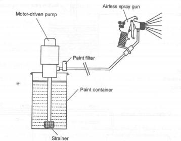
  • Airless Spray Painting (High-Pressure): Hydraulic pumps pressurize paint directly through a fine nozzle without atomizing air.

  • Cold Airless Spraying: High-pressure hydraulic pumping at ambient temperatures.

  • Hot Airless Spraying: Integrated heating element maintains paint at $70^\text{o}\text{C}\text{--}80^\text{o}\text{C}$, dropping viscosity to eliminate the need for chemical thinners.

  • Advantages: Minimal overspray, extremely rapid coverage, no air pockets, thick coat application, overhead capability.

  • Disadvantages: High equipment cost, fixed spray fan width, pronounced overlap lines, requires masking.

  • 
    

  

  • Electrostatic Spray Painting: Atomized paint particles are negatively charged in the gun nozzle and attracted to the positively charged (grounded) metal workpiece. Ensures a wrap-around effect that coats rear surfaces with up to $95\%$ paint transfer efficiency.

  • 
    

  

  • Dip Painting: Total immersion of workpieces in paint troughs, draining excess fluid in a solvent-saturated vapor zone. Ideal for complex internal channels (e.g., engine blocks), but requires large paint volumes, continuous agitation, and frequent viscosity monitoring.

• Spray Painting Defects:

  • Excessive Spray / Run: Low viscosity, excessive air pressure, or gun held too close.

  • Uneven Spray: Low air pressure, nozzle blockage, or worn spray tip.

  • Sagging: Moving gun too slowly, overly thin paint, or applying excessive paint volume.

  • Orange Peel Effect: Incorrect thinner evaporation rate, improper mixing, incorrect atomizing pressure, or dirty substrate.

Lubrication

• Primary Functions of Lubricants:

  • Reduce friction and mechanical wear between sliding or rotating surfaces.

  • Dissipate heat generated at contact zones.

  • Protect metal surfaces against chemical corrosion and environmental attack.

  • Flush away wear debris, dirt, and dynamic contaminants.

  • Seal bearing assemblies against ingress of external dust and water.

  • Absorb dynamic impact loads and damp vibrational noise.

  • Improve mechanical efficiency.

• Classification of Lubricants:

  • Solid (Dry) Lubricants: Inorganic compounds (graphite, white lead, talc/soapstone, mica, zinc oxide) used where high temperatures, extreme loads, chemical acids, or dirty environments break down liquid oils. Ideal for slides, threaded rods, locks, and hinges.

  • Semi-Solid Lubricants (Greases): Mineral or synthetic oils thickened with metal soaps (lithium, calcium, sodium). Provide long service intervals, fill dynamic clearances, and seal slow-moving, heavily loaded bearings against dust.

  • Liquid Lubricants (Oils): Fluid media suitable for high rotational speeds, light to medium loads, and continuous thermal cooling.

  • Animal Oils: Lard, tallow, sperm oil (rarely used pure due to thermal breakdown).

  • Vegetable Oils: Castor, palm, olive, linseed oils.

  • Mineral Oils: Hydrocarbons refined directly from crude petroleum.

  • Synthetic Oils: Chemically synthesized fluids (e.g., polymerized olefins) engineered for severe temperatures and extended life.

• Fluid Film Bearings & Lubrication Regimes:

  • Hydrodynamic Lubrication: Self-generating fluid pressure regime created purely by shaft rotation.

  • Stage 1: Stationary journal rests at the bottom of the bearing clearance.

  • Stage 2: Rotation begins; friction causes the journal to climb up the bearing wall.

  • Stage 3: Oil drawn into the converging wedge wedge-action generates dynamic fluid pressure, forcing the shaft down and across.

  • Stage 4: Stable equilibrium achieved; shaft floats entirely separated from the bearing shell on a continuous hydrodynamic oil wedge.

  • 
    

  

  • Hydrostatic Lubrication: External high-pressure oil pump forces lubricant directly into the bearing clearance, lifting the journal prior to and during rotation regardless of speed. Common in heavy machine tool spindles.

• Physical & Chemical Properties of Oils:

  • Viscosity: Measure of a fluid's internal resistance to shear and flow. Grade ratings dictate flow characteristics across operating temperature bands.

  • Flash Point: Minimum temperature at which an oil releases sufficient volatile vapor to ignite briefly in the presence of an open flame.

  • Fire Point: Temperature at which liberated oil vapor sustains continuous combustion (at least $5\text{ seconds}$), typically around $371^\text{o}\text{C}$.

  • Thermal Stability: Resistance of the oil structure to chemical breakdown and oxidation under prolonged exposure to high operating temperatures.

  • Oiliness: Surface-active ability of an oil to adhere to metal surfaces and maintain a continuous thin boundary layer under intense grinding pressure.

• Specialized Lubricant Types & Additives:

  • Rust & Corrosion Inhibitor Lubricants: Blended with basic polar additives to protect metallic surfaces.

  • Anti-wear Lubricants: Formulated with anti-scuffing additives for moderate sliding loads.

  • Extreme Pressure (EP) Lubricants: Contain chemical compounds (sulfur, phosphorus, chlorine) that react under high localized flash temperatures to form high-load shear layers (e.g., heavy gearboxes).

  • Monograde vs. Multigrade Oils: Monogrades suit narrow temperature ranges; Multigrades contain polymer viscosity index improvers to operate in both cold winters and hot summers (e.g., $\text{SAE } 10\text{W}-40$, where $\text{W}$ stands for winter testing rating).

• Lubricating Delivery Devices:

  • Gravity-Feed Lubricators: Drip-feed oil cups supplying continuous drops under gravity.

  • Stauffer Grease Cup: Screw-cap cup manually tightened to compress grease into bearing channels.

  • Telltale Grease Cup: Spring-loaded grease cup equipped with an indicator rod showing internal grease volume.

  • Splash Lubrication: Rotating components (crankshafts or lower gear teeth) dip into an oil sump, splashing fluid onto surrounding bearings.

Precision Measurement of Machine Parts

• Basic Instruments & Gauge Blocks:

  • Precision measurement tools include Vernier calipers, micrometers, dial test indicators, optical gauge projectors, Coordinate Measuring Machines (CMM), sine bars, precision rollers, and gauge blocks (slip gauges / Johansson blocks).

  • Slip Gauge Wringing Process: Method of sliding gauge blocks together under slight pressure with a twisting motion to eliminate air films, forming precise stack heights.

• Checking V-Grooves with Rollers and Gauge Blocks:

  • 4-Step Testing Procedure:

  • Step 1: Clean all components thoroughly and place the precision roller of known diameter into the V-groove.

  • Step 2: Calculate the theoretical stack height and assemble two identical gauge block stacks.

  • Step 3: Place the gauge block stacks on the flat top surfaces on either side of the V-groove.

  • Step 4: Place a ground straight edge horizontally across the gauge block stacks. The V-groove angle is correct if the straight edge lightly contacts the top of the precision roller without rocking and with no light showing beneath.

  • 
    

  

  • 
    

  

• Mathematical Formulae for Precision Measurement:

  • V-Groove Roller Calculation:

  • For a V-groove with included angle $2\theta$, half-angle $\theta$, depth $H_{\text{groove}}$, roller radius $R = \frac{d}{2}$, the center height $AB$ from the apex to roller center is:       $\sin(\theta) = \frac{R}{AB} \implies AB = \frac{R}{\sin(\theta)}$

  • Distance from top of roller to groove apex: $H_{\text{total}} = AB + R = R\left(1 + \frac{1}{\sin(\theta)}\right)$.

  • Checking distance $x$ above surface height $H_{\text{groove}}$: $x = H_{\text{total}} - H_{\text{groove}}$.

  • Taper Calculations Using Rollers (External Taper / Plug Gauges):

  • Half included angle $\theta$ measured using top roller diameter $D$, bottom roller diameter $d$, top measurement $M_1$, bottom measurement $M_2$, slip gauge height difference $h = H - h_0$:       $\tan(\theta) = \frac{0.5(M_1 - M_2)}{H - h_0}$

  • Included angle $= 2\theta$

  • Internal Taper Ring Gauge Measurement using Two Precision Balls:

  • 
    

  

  • Procedure: Place gauge on surface plate. Insert smaller precision ball (radius $r$) and record vertical distance to top face. Insert larger precision ball (radius $R$) and record protruding/depth height. Calculate center-to-center vertical distance $AC$. The difference in radii is $BC = R - r$. The half-angle $\theta$ satisfies:       $\sin(\theta) = \frac{R - r}{AC}$

  • Included angle $= 2\theta$

  • Sine Bar Principles & Formulae:

  • High-precision chromium-steel bar containing two ground cylinders of equal diameter separated by accurate center distance $l$ (typically $100\,mm$ or $200\,mm$).

  • 
    

  

  • 
    

  

  • Formula: For stack height difference $h = H_2 - H_1$ and sine bar length $l$:       $\sin(\theta) = \frac{h}{l} \implies \theta = \arcsin\left(\frac{h}{l}\right)$

  • Included angle $i = 2\theta$

• Detailed Worked Examples:

  • Example 1 (Internal Taper with Two Balls):

  • Given: Top ball diameter $D = 30\,mm$ ($R = 15\,mm$), bottom ball diameter $d = 20\,mm$ ($r = 10\,mm$), total height to top ball crown $36.75\,mm$, protrusion of top ball $4.25\,mm$.

  • $BC = R - r = 15 - 10 = 5\,mm$

  • Vertical distance between centers $AB = 36.75 + 10 - 4.25 - 15 = 27.5\,mm$

  • $\sin(\theta) = \frac{BC}{AB} = \frac{5}{27.5} = 0.1818$\implies \theta = \arcsin(0.1818) = 10.486^\text{o}\n - Included angle 2\theta = 20.972^\text{o}\n\n - *Example 2 (Tapered Hole Depth Calculation):*\n - Given: Hole top diameter 20\,mm$, included angle$30^\text{o}$(half-angle$\theta = 15^\text{o}$), ball diameter$d = 12\,mm$($r = 6\,mm).\n - \sin(15^\text{o}) = \frac{r}{AB} = \frac{6}{AB} \implies AB = \frac{6}{\sin(15^\text{o})} = 23.182\,mm\n - Distance from top face to apex DE = \frac{10}{\tan(15^\text{o})} = 37.321\,mm\n - Relationship: DE = x + r + AB \implies 37.321 = x + 6 + 23.182\n - Protrusion / depth distance x = 37.321 - 29.182 = 8.139\,mm\n\n - *Example 3 (External Dovetail Distance Between Rollers):*\n - Given: Overall width across bottom corners 125\,mm$, dovetail angle$45^\text{o}$, roller diameter$15\,mm$($R = 7.5\,mm).\n - Half angle for bottom corner contact \beta = \frac{45^\text{o}}{2} = 22.5^\text{o}\n - Horizontal distance from corner to roller center AB = \frac{R}{\tan(22.5^\text{o})} = \frac{7.5}{\tan(22.5^\text{o})} = 18.107\,mm\n - Distance across inside faces X = 125 - 2(R) - 2(AB) = 125 - 2(7.5) - 2(18.107) = 73.786\,mm\n\n# Gear Drives\n\n- **Advantages of Gear Drives:**\n - Positive, non-slip power transmission.\n - High efficiency and direct power delivery.\n - Extremely compact physical design.\n - Capability to transmit high loads and heavy torque.\n - Low radial shaft loads compared to tight belt drives.\n - Minimal maintenance required under proper lubrication.\n\n- **Spur Gear Terminology:**\n - **Pitch Circle Diameter (PCD):** The diameter of the imaginary pitch cylinder that rolls without slipping with the pitch cylinder of a meshing gear.\n - **Module (m$):** Ratio of pitch circle diameter to the number of teeth ($m = \frac{\text{PCD}}{T}), expressed in millimeters.\n - **Circular Pitch (CP$):** Distance measured along the pitch circle circumference between corresponding points of adjacent teeth ($CP = \pi \times m).\n - **Addendum:** Radial distance from pitch circle to top of tooth (\text{Addendum} = m).\n - **Dedendum:** Radial distance from pitch circle to bottom root circle (\text{Dedendum} = 1.25 \times m).\n - **Total Tooth Depth:** Sum of addendum and dedendum (\text{Total Depth} = 2.25 \times m).\n - **Tooth Thickness:** Circular length along pitch circle (\text{Thickness} = \frac{CP}{2} = \frac{\pi m}{2}).\n - **Outside Diameter (D_o$):** Total diameter over tooth tips ($D_o = m(T + 2)).\n - **Centre Distance (C$):** Distance between center axes of meshing external gears ($C = \frac{m(T_A + T_B)}{2}$). For internal meshing ring gears:$C = \frac{m(T_B - T_A)}{2}.\n - **Velocity Ratio (VR$):** Ratio of driver rotational speed to driven rotational speed ($VR = \frac{N_A}{N_B} = \frac{T_B}{T_A} = \frac{\text{PCD}B}{\text{PCD}_A}).\n\n- **Simple and Compound Gear Trains:**\n - Pitch line velocity for gears in mesh is identical: v = \frac{\pi \times \text{PCD}_A \times N_A}{60} = \frac{\pi \times \text{PCD}_B \times N_B}{60}.\n - Therefore, T_A \times N_A = T_B \times N_B\n - **Compound Gear Train Equation:**\n    \frac{N{\text{output}}}{N_{\text{input}}} = \frac{\prod \text{Number of Teeth on Driving Gears}}{\prod \text{Number of Teeth on Driven Gears}}\n\n- **Epicyclic Gear Drives:**\n - Gear systems containing orbiting planet gears mounted on a rotating carrier arm that revolve around a central sun gear and mesh inside an internal ring gear (annulus).\n - Tooth relationship rule for standard planetary arrangement: T_{\text{Annulus}} = T_{\text{Sun}} + 2 \times T_{\text{Planet}}.\n - **Tabular Method of Analysis:**\n\n    | Condition / Step | Arm D$| Sun Gear$S$| Planet Gear$P$| Ring Gear / Annulus$A |\n    | :--- | :--- | :--- | :--- | :--- |\n    | **1. Fix Arm D$, rotate$A$by$+1$rev** |$0$|$+\frac{T_A}{T_S}$|$-\frac{T_A}{T_P}$|$+1 |\n    | **2. Multiply across by x$** |$0$|$+x \left(\frac{T_A}{T_S}\right)$|$-x \left(\frac{T_A}{T_P}\right)$|$+x |\n    | **3. Add y$to all columns** |$y$|$x \left(\frac{T_A}{T_S}\right) + y$|$-x \left(\frac{T_A}{T_P}\right) + y$|$x + y |\n\n- **Worked Epicyclic Example:**\n - Given: Sun gear T_S = 40$, Planet gear$T_P = 20$, Annulus$T_A = 40 + 2(20) = 80$. Sun gear input speed$N_S = +300\text{ r/min} (clockwise).\n - *Case (a):* Annulus fixed (N_A = 0$). Calculate output arm speed$N_{\text{Arm}} = y$.

  • From Annulus column: $x + y = 0 \implies x = -y$

  • From Sun column: $-2x + y = N_S \implies -2(-y) + y = 300 \implies 3y = 300 \implies y = 100\text{ r/min}$.

  • Output arm rotates at $100\text{ r/min}$ Clockwise.

  • Case (b): Arm rotates at $-10\text{ r/min}$ (counter-clockwise, $y = -10$), Sun gear at $+300\text{ r/min}$. Calculate Annulus speed $N_A$.

  • From Sun column: $-2x + (-10) = 300 \implies -2x = 310 \implies x = -155$

  • From Annulus column: $N_A = x + y = -155 + (-10) = -165\text{ r/min}$.

  • Annulus rotates at $165\text{ r/min}$ Counter-Clockwise.

Belt Drives

• Types of Belts & Drives:

  • Flat Belts: Made of leather or synthetic rubber/ply composite; used for long center distances; higher slip risk.

  • V-Belts / Wedge Belts: Trapezoidal cross-section fitting into wedged pulley grooves (groove angle $32^\text{o}\text{--}38^\text{o}$, belt included angle $40^\text{o}$). Wedging action eliminates slip.

  • Conveyor Belts: Heavy-duty multi-ply belts backed by cotton/nylon layers designed to carry bulk material across inclined spans.

• Geometrical Equations & Lap Angles:

  • Effective Diameter ($D_E$): $D_E = D_{\text{pulley}} + t_{\text{belt}}$.

  • Open Drive Configuration:

  • Both pulleys rotate in the same direction.

  • Half wrap offset angle $\alpha$: $\sin(\alpha) = \frac{D_E - d_E}{2C}$

  • Contact angle on small pulley: $\theta_{\text{small}} = 180^\text{o} - 2\alpha$ (in degrees) $= (180^\text{o} - 2\alpha) \times \frac{\pi}{180^\text{o}}$ (in radians).

  • Contact angle on large pulley: $\theta_{\text{large}} = 180^\text{o} + 2\alpha$.

  • Belt length: $L = \frac{\pi}{2}(D_E + d_E) + \frac{(D_E - d_E)^2}{4C} + 2C$.

  • Crossed Drive Configuration:

  • Pulleys rotate in opposite directions.

  • $\sin(\alpha) = \frac{D_E + d_E}{2C}$

  • Contact angle identical on both pulleys: $\theta = 180^\text{o} + 2\alpha$.

  • Belt length: $L = \frac{\pi}{2}(D_E + d_E) + \frac{(D_E + d_E)^2}{4C} + 2C$.

• Tension Dynamics & Power Equations:

  • Belt Velocity ($v$): $v = \frac{\pi \times D_E \times N}{60}\quad (\text{m/s})$.

  • Centrifugal Tension ($T_c$): Extra tension pulling belt away from pulley at high speeds ($v > 10\,m/s$):     $T_c = m \times v^2 = (\rho \times A) \times v^2$     Where $m$ is mass per unit length ($kg/m$), $\rho$ is density ($kg/m^3$), $A = w \times t$ is cross-sectional area ($m^2$).

  • Tension Ratio Equations:

  • Flat Belts: $\frac{T_1 - T_c}{T_2 - T_c} = e^{\mu \theta}$

  • V-Belts (Groove half angle $\beta$): $\frac{T_1 - T_c}{T_2 - T_c} = e^{\frac{\mu \theta}{\sin(\beta)}}$

  • Maximum Tensile Stress Constraint: $T_1 = \sigma_{\text{max}} \times A = \sigma_{\text{max}} \times (w \times t)$.

  • Power Transmission ($P$):

  • Single belt: $P = (T_1 - T_2) \times v$

  • Multi-belt / Multi-ply drive: $P = (T_1 - T_2) \times v \times n_{\text{belts}}$

  • Torque ($T$) & Shaft Reaction:

  • Torque $T = (T_1 - T_2) \times r$

  • Total force on bearings $F_B = T_1 + T_2 + W_{\text{pulley}}$.

• Conveyor Belt Systems:

  • Power Components:

  • Power required to overcome gravity: $P_g = m_{\text{mass flow}} \times g \times h$ (where $m_{\text{mass flow}}$ is in $kg/s$, $h$ is vertical lift height).

  • Power required to overcome friction: $P_f = F_f \times v$

  • Total Head Pulley Power: $P_H = P_g + P_f = (T_1 - T_2) \times v$

  • Motor Input Power: $P_{\text{motor}} = \frac{P_H}{\eta}$.

  • Mass Flow Unit Conversion:

  • To convert $\text{tonne/hour}$ to $kg/s$: divide by $3.6$

  • To convert $kg/s$ to $\text{tonne/hour}$: multiply by $3.6$

• Worked Belt Drive Example:

  • Given: V-belt drive transmitting $30\,kW$, pulley effective diameter $D_E = 200\,mm$ ($0.2\,m$), speed $N = 600\text{ r/min}$, groove included angle $2\beta = 40^\text{o}$ ($\beta = 20^\text{o}$), lap angle $\theta = 150^\text{o} = 2.618\text{ rad}$, coefficient of friction $\mu = 0.3$, belt unit mass $m = 0.6\,kg/m$, max allowable tension per belt $T_1 = 700\,N$.

  • $v = \frac{\pi \times 0.2 \times 600}{60} = 6.283\,m/s$

  • $T_c = m \times v^2 = 0.6 \times (6.283)^2 = 23.686\,N$

  • $\frac{\mu \theta}{\sin(\beta)} = \frac{0.3 \times 2.618}{\sin(20^\text{o})} = \frac{0.7854}{0.3420} = 2.296$

  • $e^{2.296} = 9.938$

  • $\frac{700 - 23.686}{T_2 - 23.686} = 9.938 \implies \frac{676.314}{T_2 - 23.686} = 9.938 \implies T_2 = 91.739\,N$

  • Power per single belt $P_{\text{single}} = (T_1 - T_2) \times v = (700 - 91.739) \times 6.283 = 3821.7\,W$

  • Number of belts needed $n = \frac{30000}{3821.7} = 7.85 \implies 8\text{ belts}$.

Hydraulic Systems

• Fluid Fundamentals & Physical Constants:

  • Density of Water: $\rho_{\text{water}} = 1000\,kg/m^3$.

  • Density of Mercury: $\rho_{\text{Hg}} = 13600\,kg/m^3$.

  • Relative Density of Mercury: $S_{\text{Hg}} = 13.6$.

  • Acceleration due to gravity: $g = 9.81\,m/s^2$.

  • Volumetric Flow Rate: $Q = A \times v\quad (m^3/s)$.

  • Mass Flow Rate: $m = \rho \times Q\quad (kg/s)$.

• Bernoulli's Energy Equation:

  • In an ideal, incompressible fluid flow without friction losses, total energy per unit weight remains constant along a streamline:     $\frac{P}{\rho g} + \frac{v^2}{2g} + z = \text{Constant}$     Where $\frac{P}{\rho g}$ is Pressure Head ($m$), $\frac{v^2}{2g}$ is Velocity / Kinetic Head ($m$), and $z$ is Potential / Elevation Head ($m$).

• Flow Through Orifices & Vena Contracta:

  • Orifice Plate: Circular opening in a plate causing fluid streamlines to converge to a minimum cross-sectional area called the Vena Contracta downstream of the orifice edge.

  • Theoretical Velocity ($v_t$): $v_t = \sqrt{2gh}$.

  • Hydraulic Coefficients:

  • Coefficient of Velocity ($C_v$): Ratio of actual velocity at vena contracta to theoretical velocity ($C_v = \frac{v_a}{v_t}$). Measured via jet trajectory ($x$ horizontal, $y$ vertical drop): $v_a = \frac{x}{\sqrt{\frac{2y}{g}}} \implies C_v = \frac{x}{2\sqrt{yh}}$.

  • Coefficient of Contraction ($C_c$): Ratio of vena contracta area to orifice area ($C_c = \frac{A_a}{A_t} = \frac{d_a^2}{d_t^2}$).

  • Coefficient of Delivery / Discharge ($C_d$): Ratio of actual discharge to theoretical discharge ($C_d = \frac{Q_a}{Q_t} = C_v \times C_c$).

  • Head Loss Due to Fluid Friction:     $h_L = h \left(1 - C_v^2\right) = h - \frac{v_a^2}{2g}$

• Venturi Meters & Differential Pressure:

  • Device consisting of a converging cone, narrow throat, and diverging cone used to measure pipe flow.

  • Actual Discharge Equation:     $Q_a = C_d \times \frac{A_1 A_2}{\sqrt{A_1^2 - A_2^2}} \times \sqrt{2gh}$     Where $A_1$ is pipe area, $A_2$ is throat area, $h$ is equivalent head of fluid flowing.

  • U-Tube Mercury Manometer Equivalent Head Conversion:     $h_{\text{water}} = \left(\frac{\rho_{\text{Hg}}}{\rho_{\text{water}}} - 1\right) \times h_{\text{Hg}} = (13.6 - 1) \times h_{\text{Hg}} = 12.6 \times h_{\text{Hg}}$

• Pipeline Friction Losses:

  • Darcy-Weisbach Equation:     $h_f = \frac{4 f L v^2}{2g d} = \frac{f L Q^2}{3.026 d^5}$     Where $f$ is Darcy's friction coefficient, $L$ is pipe length, $d$ is pipe inner diameter.

  • Chezy Equation:     $v = C \sqrt{m \cdot i}$     Where $C$ is Chezy's constant, $m = \frac{\text{Area}}{\text{Wetted Perimeter}} = \frac{d}{4}$ (for full round pipe), $i = \frac{h_f}{L}$ is hydraulic gradient.

Bearings

• Classification & Load Types:

  • Rolling Element Bearings: Ball bearings, roller bearings, needle bearings, taper roller bearings. Feature low friction, standardized dimensions, and easy replacement.

  • Load Configurations:

  • Radial Load ($F_r$): Forces acting perpendicular to shaft axis.

  • Axial / Thrust Load ($F_a$): Forces acting parallel along shaft axis.

  • Angular / Combined Load: Simultaneous combination of radial and axial load vectors.

  • Static vs. Dynamic Loads: Static loads remain constant without movement; Dynamic loads vary continuously in magnitude and direction over operating time (causing fatigue).

• Forces on Spur Gears Transmitted to Bearings:

  • For a gear delivering torque $T$ with pitch circle diameter $\text{PCD}$ and pressure angle $\alpha = 20^\text{o}$:

  • Tangential force: $F_T = \frac{2T}{\text{PCD}}$

  • Separating Radial force: $F_R = F_T \times \tan(20^\text{o})$

  • Total Normal force: $F_N = \frac{F_T}{\cos(20^\text{o})}$

• Fluctuating Loads & Mean Equivalent Load ($F_m$):

  • Stepped Load: $F_m = \left[ \frac{F_1^p n_1 t_1 + F_2^p n_2 t_2 + \dots + F_n^p n_n t_n}{n_1 t_1 + n_2 t_2 + \dots + n_n t_n} \right]^{1/p}$     (Where exponent $p = 3$ for ball bearings, $p = \frac{10}{3}$ for roller bearings).

  • Linear / Sinusoidal Fluctuating Load:

  • $F_m = \frac{F_{\text{min}} + 2 F_{\text{max}}}{3}$ (standard linear approximation).

• Static and Dynamic Equivalent Loads:

  • Static Equivalent Radial Load: $F_{0q} = X_0 F_r + Y_0 F_a$

  • Dynamic Equivalent Radial Load: $P_r = X F_r + Y F_a$     (Where $X$ and $Y$ are radial and axial load factors from manufacturer tables).

• Basic Rating Life ($L_{10}$ and $L_{10h}$):

  • ISO formula for basic rating life in millions of revolutions with $90\%$ reliability:     $L_{10} = \left(\frac{C_r}{P_r}\right)^p$     Where $C_r$ is basic dynamic load rating ($N$), $P_r$ is dynamic equivalent load ($N$), $p = 3$ (ball) or $p = \frac{10}{3}$ (roller).

  • Rating life in operating hours ($L_{10h}$) at constant speed $n\text{ (r/min)}$:     $L_{10h} = \frac{10^6}{60 \times n} \times \left(\frac{C_r}{P_r}\right)^p$

• Worked Bearing Calculation:

  • Given: Roller bearing ($p = \frac{10}{3}$), required life $L_{10h} = 1400\text{ hours}$, operating speed $n = 800\text{ r/min}$, dynamic equivalent load $P_r = 1037\,N$. Calculate $C_r$

  • $1400 = \frac{10^6}{60 \times 800} \times \left(\frac{C_r}{1037}\right)^{10/3}$

  • $1400 = 20.8333 \times \left(\frac{C_r}{1037}\right)^{10/3}$

  • $\left(\frac{C_r}{1037}\right)^{10/3} = \frac{1400}{20.8333} = 67.200$

  • $\frac{C_r}{1037} = (67.200)^{3/10} = (67.200)^{0.3} = 3.534$

  • $C_r = 3.534 \times 1037 = 3664.8\,N\quad (3.665\,kN)$.

Metal Cutting Machines

• General Kinetic Formulae:

  • Force $F = m \times a$

  • Weight $W = m \times g$

  • Torque $T = F \times r$

  • Cutting Velocity $v = \frac{\pi \times D \times N}{60}\quad (m/s)$

  • Work Done $W_D = F \times s$

  • Power $P = \frac{W_D}{t} = F \times v = \frac{2\pi N T}{60}$

  • Mechanical Efficiency $\eta = \frac{P_{\text{output}}}{P_{\text{input}}} \times 100\%$

  • Friction Force $F_f = \mu \times W$

  • Frictional Power Loss $P_f = F_f \times v$

• Machine Vices & Work Holding:

  • Horizontal friction holding force: $F_{\text{horizontal}} = \mu \times F_{\text{clamping}}$.

• Shaping Machines:

  • Reciprocating machine tool cutting flat surfaces or keyways using a single-point tool.

  • Total cutting stroke distance in time $t$: $s = \text{Strokes/min} \times L_{\text{stroke}} \times t_{\text{min}}$.

  • Total Work Done $W_D = F_{\text{cutting}} \times s$

  • Power Consumed $P = \frac{W_D}{t_{\text{seconds}}}$.

• Centre Lathes:

  • Workpiece rotates while single-point tool feeds linearly.

  • Cross-sectional area of cut $A_{\text{cut}} = D_{\text{cut}} \times f$ (where $D_{\text{cut}}$ is depth of cut in $mm$, $f$ is feed per revolution in $mm/\text{rev}$).

  • Tangential Cutting Force $F_{\text{cut}} = p_{\text{cut}} \times A_{\text{cut}} = p_{\text{cut}} \times D_{\text{cut}} \times f$ (where $p_{\text{cut}}$ is specific cutting pressure in $N/mm^2$ or $MPa$).

  • Useful Cutting Power $P_{\text{useful}} = F_{\text{cut}} \times v = \frac{2\pi N T}{60}$.

  • Total Motor Input Power $P_{\text{input}} = \frac{P_{\text{useful}}}{\eta}$.

• Milling Machines:

  • Multi-tooth rotating cutter removes material as table feeds workpiece.

  • $P_{\text{cutter}} = \eta \times P_{\text{motor}}$.

• Drilling Machines:

  • Rotating drill bit performs drilling, countersinking, counterboring, reaming, or tapping.

  • Torque $T = F \times r$, Power $P = \frac{2\pi N T}{60}$.

• Surface Grinding Machines:

  • High-speed abrasive wheel grinds flat surfaces on workpieces held by an electromagnetic chuck.

  • Total downforce on workpiece $F_{\text{vertical}} = W_{\text{workpiece}} + F_{\text{magnetic}}$.

  • Maximum allowable horizontal cutting force without slippage: $F_{\text{horizontal}} = \mu \times F_{\text{vertical}} = \mu (m g + F_{\text{magnetic}})$.

• Worked Lathe Power Calculation:

  • Given: Workpiece diameter $D = 50\,mm$ ($0.05\,m$), rotational speed $N = 1400\text{ r/min}$, depth of cut $D_{\text{cut}} = 3\,mm$, feed $f = 1.5\,mm/\text{rev}$, specific cutting pressure $p_{\text{cut}} = 1200\,N/mm^2$, friction losses $= 30\%$ (efficiency $\eta = 70\% = 0.7$).

  • Cutting speed $v = \frac{\pi \times 0.05 \times 1400}{60} = 3.665\,m/s$

  • Area of cut $A = 3 \times 1.5 = 4.5\,mm^2$

  • Cutting Force $F = 1200 \times 4.5 = 5400\,N$

  • Useful Output Power $P_{\text{out}} = F \times v = 5400 \times 3.665 = 19791\,W$

  • Total Input Power $P_{\text{in}} = \frac{19791}{0.7} = 28273\,W\quad (28.273\,kW)$.