5. Factors affecting threshold: Instrument Factors
Instrument Factors
Thresholds in visual field testing are influenced by both the instrument and the patient.
Important to differentiate reduced sensitivity due to pathology from reductions caused by patient (physiological) or instrument variables.
Background Luminance
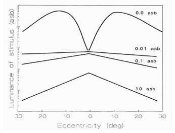
Sensitivity depends on background illumination according to Weber's Law.
Weber's Law: where (I) is background luminance and (\Delta I) is the just-noticeable change in luminance.
Background luminance values used in practice:
Humphrey perimetry:
Medmont:
This difference corresponds to a ~ difference in background intensity.
Both are in the photopic range.
Stimulus Size
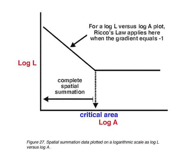
Visual field sensitivity varies with stimulus size, described by Ricco's Law.
Ricco's Law (small stimuli): for small stimulus areas, the product of stimulus luminance and stimulus area at threshold is constant.
In formula form: for a given threshold, where (L) is luminance and (A) is stimulus area; this holds up to a critical area.
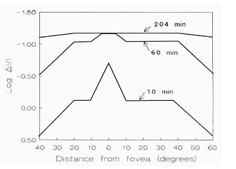
Practical implication: stimulus size affects detectability and measured sensitivity.
Hill of vision has a higher peak but at lower sensitivity for smaller stimulus size.
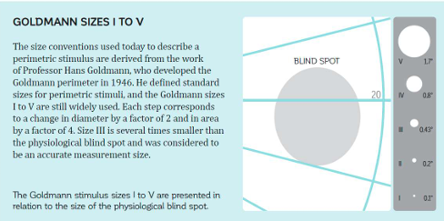
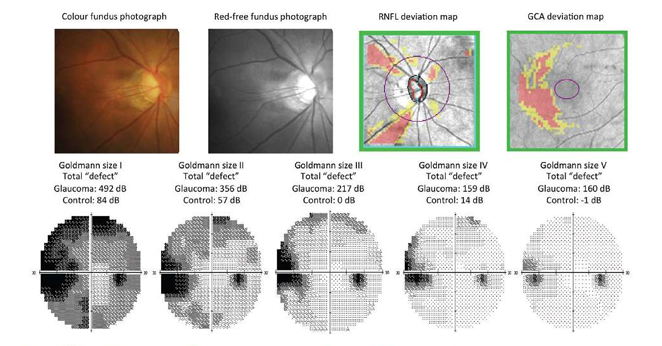
Stimulus Size – Goldmann Sizes I–V
Goldmann stimulus sizes and their approximate physical properties:
I: Area ; Degrees
II: Area ; Degrees
III: Area ; Degrees
IV: Area ; Degrees
V: Area ; Degrees
Goldmann size notation is a standard way to specify stimulus size in perimetry
Size III is standard size (most commonly used for normative data)
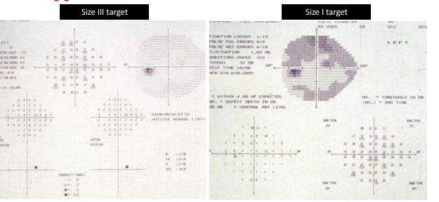
Stimulus Size – Advantages of Small Stimuli
Small stimuli provide higher spatial resolution, making it easier to detect small defects.
When used with a finer testing grid, small stimuli (e.g., Size III vs Size I) improve defect localization and mapping.
The accompanying figure (from the source) contrasts results using different sizes, illustrating how small targets can reveal subtle defects earlier.
Stimulus Size – Large Stimuli Advantages
Large stimuli yield advantages such as:
Defocus has less effect on detection
Greater dynamic range for detecting defects
better representation of px view / functional range.
Stimulus Size – Large vs Small: practical takeaway
Smaller stimuli improve resolution and defect detection on finer grids.
Larger stimuli provide more robustness to defocus and yield broader dynamic ranges for detecting defects.
Short Wavelength Automated Perimetry (SWAP)
SWAP targets the koniocellular pathway by stimulating short-wavelength (blue) cones.
Key characteristics:
Targets the koniocellular pathway projecting from blue-on cells in the retina.
Temporal and spatial properties differ from the parvocellular pathway tested by White-on-White perimetry (SAP).
Topography of SWAP fields is different from SAP fields.
Test stimulus and background:
Uses a large blue target (size V).
Peak wavelength: to stimulate SWS cones.
Background is bright yellow: .
Targets are larger due to the lower stimulus brightness and to test koniocellular ganglion cells.
Isolation of B pathway:
SWAP saturates G (green), R (red) and rod pathways to isolate the B (koniocellular) pathway.
Availability:
Implemented on some Humphrey Field Analyzers (HFA), plus Oculus and Octopus models.
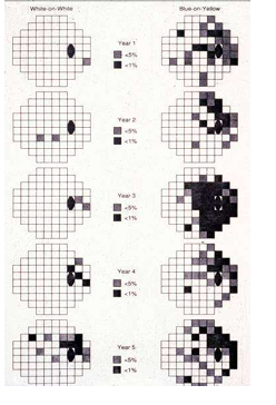
SWAP – Early clinical observations
Early reports suggested:
Up to of optic nerves are lost before field defects manifest on SAP.
SWAP reveals deeper VF defects in glaucoma patients than SAP.
SWAP defects may precede SAP defects by .
SWAP defects can be predictive of the onset and location of future SAP field loss.
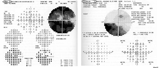
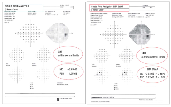
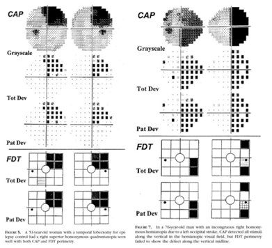
SWAP – Case examples and interpretation
Case where SWAP shows a defect with SAP normal (illustrative): SWAP defect can exist even when SAP is normal, highlighting SWAP's potential for earlier detection.
Example data (from a single-field SWAP case)
Example results include pattern deviation (PD) and total deviation (TD) metrics with fixation monitoring and fixation losses (often 0/12 or similar).
SWAP data often include PSD (pattern standard deviation) and MD (mean deviation) values that help quantify defect severity.
SWAP – Practical considerations and limitations
Advantages:
Ability of SWAP to detect defects earlier explained by the reduced redundancy theory
Relatively few koniocellular cells (<15% of cell population)
Hence there is less redundancy that can potentially mask VF defects
Some studies have reported that SWAP is useful in identifying VF defects due to diabetic retinopathy, macular oedema and neuro ophthalmological disorders
SITA-Swap now available
3-6 minute test time > 1/3 faster than standard SWAP
Disadvantages:
Affected by media opacities (e.g., lens opacities/cataracts).
Higher within- and between-observer variability compared with SAP.
10-2 SWAP testing: Some evidence suggests SWAP 10-2 could be useful for detecting paracentral (central) defects in pre-perimetric glaucoma.
Jung et al. (2015) cited.
Frequency Doubling Perimetry (FDT)
Purpose and mechanism:
Function-specific test that isolates a subpopulation of retinal ganglion cells (primarily magnocellular, M-cells) to identify early visual field defects.
Uses a frequency-doubling illusion: a low spatial frequency sine grating (<1 cycle/degree) flickering in counter-phase at a high temporal frequency (>15 Hz).
flickering target rather than a spot target.
Spatial frequency appears doubled, yielding a high-contrast detection task for M-cells (3%–9% contrast).
Evidence suggests M-cells are damaged first in glaucoma.
Test design and stimuli:
Uses patterns similar to Humphrey Field Analyzer (30-2, 24-2, 10-2, and macula threshold).
Patient responds to flicker of black-white bars rather than the mere presence of a stimulus.
Reliability and indices:
Reliability indices include fixation monitoring (Heijl-Krakau method), false positives (FP), and false negatives (FN).
Age-matched indices: MD, PSD, GHT (glaucomatous hemifield test).
ADVANTAGE:
Due to low spatial frequency stimuli, FDT sensitivity is not affected by optical blur (even with higher ametropia, roughly ±6 diopters), pupil size, or ambient illumination.
FDT – Test patterns and results
Common test patterns include: 30-2, 24-2, 10-2, and macula threshold.
Test duration and efficiency:
FDT uses a rapid Bayesian-like algorithm (Zippy estimates of sequential testing) to reduce test time to about 4 minutes
Normative database:
Includes about individuals aged to years.
Efficacy in glaucoma detection:
Studies indicate FDT 24-2 is superior for detecting glaucomatous field loss, especially in early disease
but may be less reliable for detecting neurological defects
Comparative spatial characterization:
Some studies (e.g., Matrix 30-2) suggest improvements in spatial pattern characterization over standard FDT 30-2.
FDT – Practical conclusion
FDT perimetry is useful for detecting glaucomatous visual field changes, particularly in early disease, but it may be less reliable for identifying neurological defects.