Simple Linear Regression & Multiple Linear Regression

Definition (#f7aeae)

Important (#edcae9)

Extra (#fffe9d)

Regression:

Overview: 2*

• Regression uses exactly the same data as that used by correlation.

  • Correlation: Considers how closely the data points fall to the line of best fit.

  • Regression: Describes the characteristics of the straight line.

• Uses both the slope of the line as well as the point it intercepts the y-axis.

• Develops a regression equation to predict the y value based on the x value.

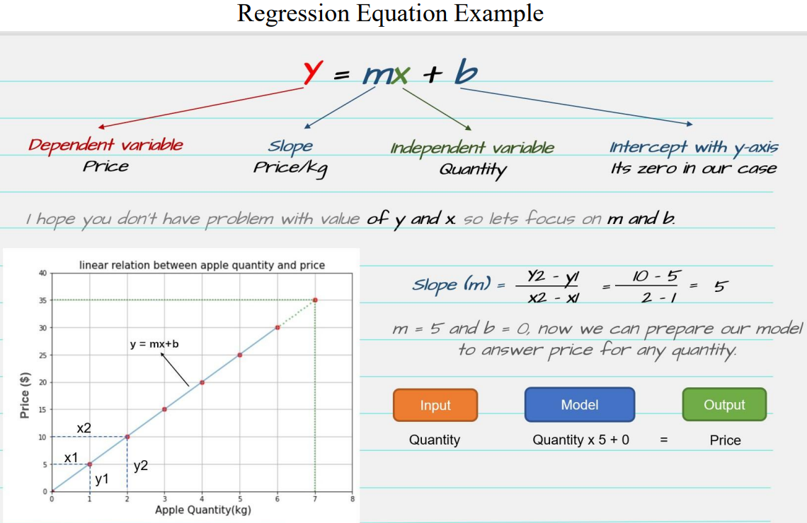
Regression equation: 1*

To calculate a regression line:

• Intercept (b): The point at which the line cuts across the y-axis.

• The slope of the regression line; normally denoted by the letter (m).

  • The slope: The number of units that the regression line moves up the vertical axis for each unit of movement along the horizontal axis.

• Y = mX + b

• m: Estimated slope.

• b: Estimated intercept.

• X: The predictor (independent) variable.

• Y: The response (dependent) variable.

Simple Linear Regression:

Overview: 3*

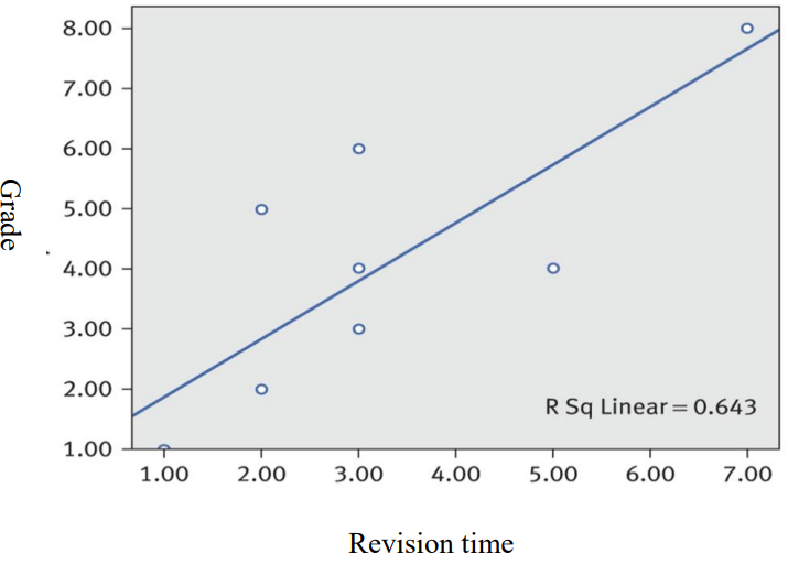
• 1 predictor and 1 outcome.

  • Forms a linear relationship.

• Provides the line of best fit.

• The variance explained can be attributed directly to the predictor.

Assumptions: 3*

1. Linearity:

   • The relationship between the IV (X) and DV (Y) should be linear.

   • The data points should form a straight-line pattern when plotted.

2. Independence of errors:

   • The residuals (differences between observed and predicted values) must be independent.

   • No autocorrelation, meaning no pattern in residuals over time or order.

3. Homoscedasticity:

   • The variance (spread) of residuals should be constant across all levels of the independent variable.

   • No fan-shaped or cone-shaped pattern in residual plots

4. Normality of residuals:

   • Residuals should be approximately normally distributed, especially for making inferences (hypothesis testing).

Analysis:

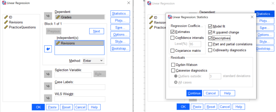
1. Analyze → Regression→ Linear.

2. Put outcome in “Dependent”. Put predictor in “Independent”.

3. Click “Statistics” → Tick “R squared change”, “Descriptive”, and “Part and partial correlation → Click “continue”.

4. Click “OK”

   

Interpretation:

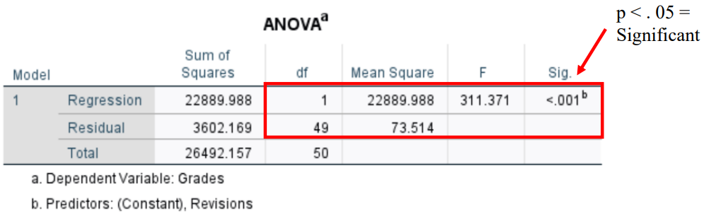
1. If sig (p) <.05, predictor significantly predicts outcome.

   • If sig (p) >.05, there is no significant relation. (ANOVA table).

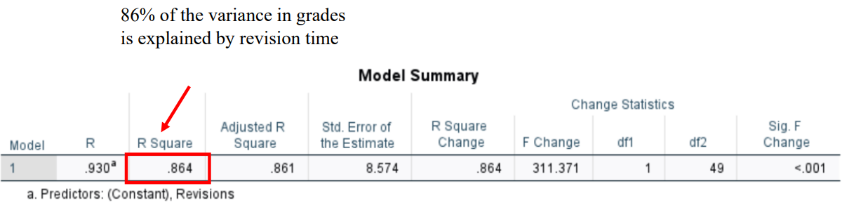
2. See R² to see how much variance in the outcome is explained the predictor. (Model summary table).

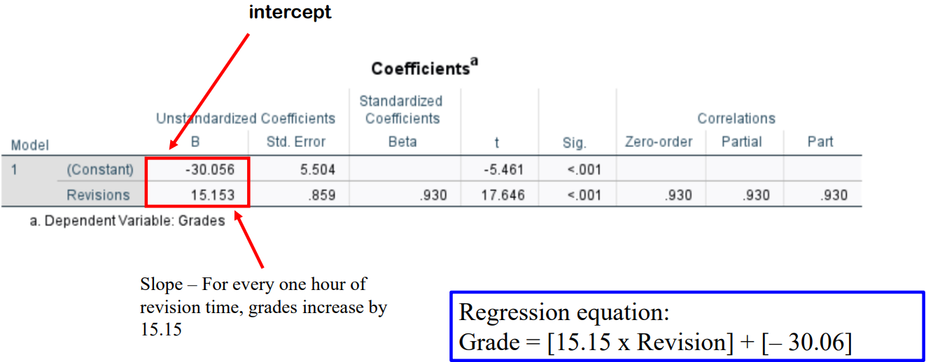
3. See “B” under “unstandardized coefficients”. “Constant” is the intercept for the equation.

   • The IV is the regression coefficient/slope. (Coefficient table)

Output: 3*

Research question: 2*

Template:

• What test you ran and why & what variables were plugged in.

• Is there a significant prediction.

  • If yes, report the variance.

• Report the “equation” above with the values.

• Interpretation:

• If significant: When predictor increases by 1 unit, what happened to the outcome.

• If not significant: No relation.

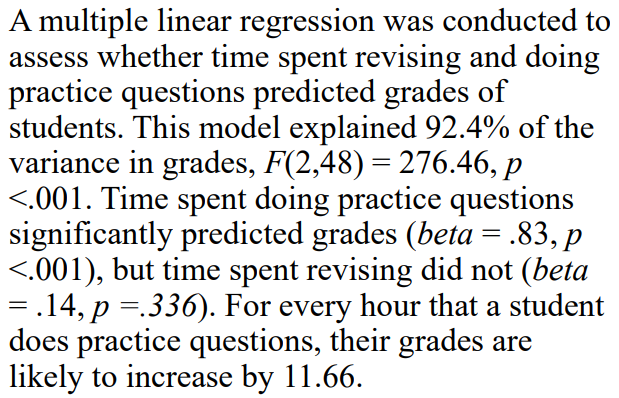
Multiple Linear Regression:

Overview: 3*

• More than 1 predictor and 1 outcome.

  • Forms a regression model.

• Provides plane of best fit.

• The variance explained reflects the total from the predictors as a whole.

• Beta weights are used to determine how much each respective predictor contributes.

Assumptions: 3*

1. Linearity:

   • The relationship between each IV and the DV should be linear.

   • Check this assumption using scatterplots for each predictor.

2. Independence of errors:

   • The residuals must not be correlated.

   • No patterns in residual plots over time, and data points should be independent.

3. Homoscedasticity:

   • Residuals should have constant variance across all levels of the predictors.

   • Look for consistent spread of residuals in a plot.

4. Normality of residuals:

   • Residuals should follow a normal distribution.

   • Normality is checked through histograms or Q-Q plots of residuals.

5. No multicollinearity:

   • The IV’s should not be highly correlated with each other.

   • High correlation among predictors can distort results and make the model less reliable.

Equation:

• Y = m1X1 + m2X2 +m3X3 + b

• m1: The slope of Predictor 1.

• m2: The slope of Predictor 2 .

• m3: The slope of Predictor 3.

• b: The intercept.

• X1,X2,X3 = Predictors.

• Y: The outcome (dependent) variable.

Analysis:

1. Same steps as simple linear regression.

2. Put all the predictors into the “Independent” space

Interpretation:

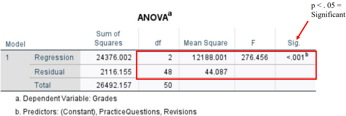
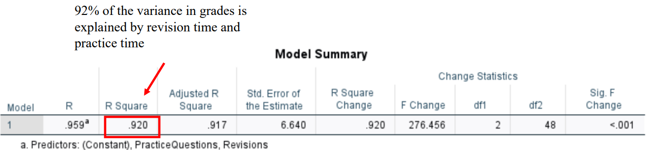
1. If sig (p) <.05, predictors significantly predicts outcome as a whole.

   • If sig (p) >.05, there is no significant relation. (ANOVA table).

2. See R² to see how much variance in the outcome is explained all the predictors. (Model summary table).

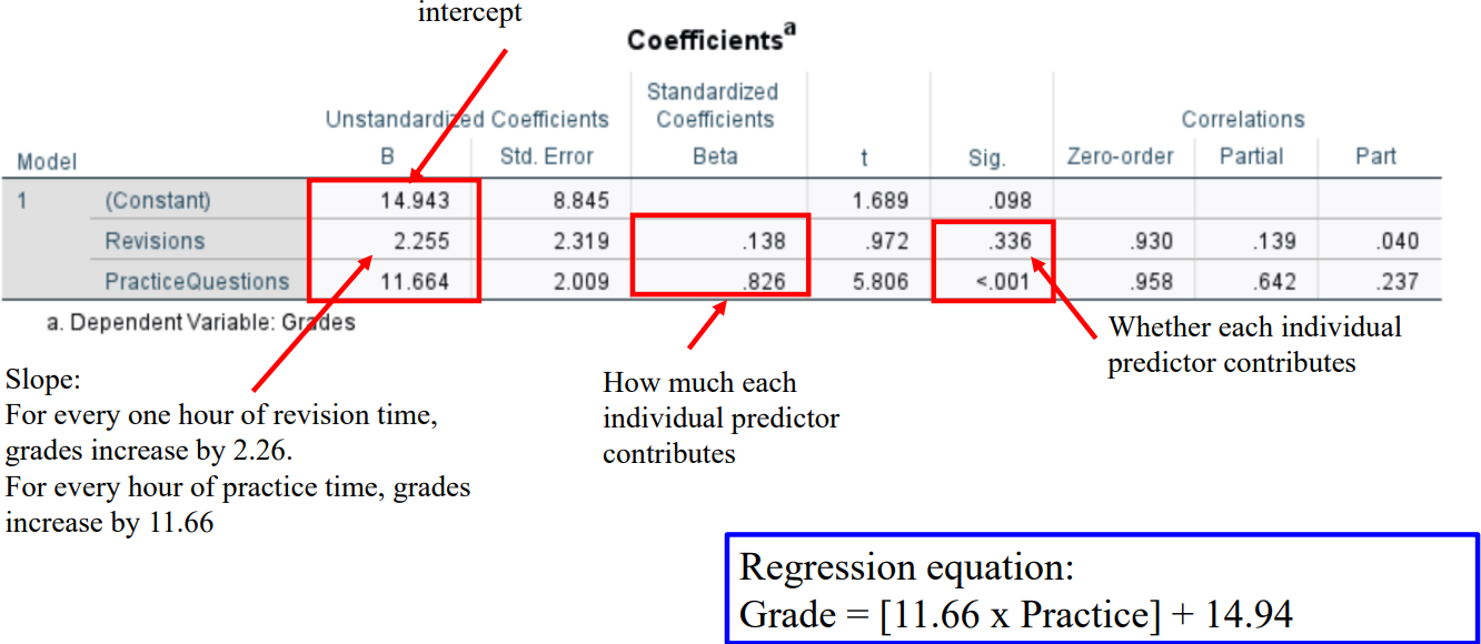
3. The sig shows which predictor is significant, and which is not. (Coefficient table).

4. See “Beta” under “standardized coefficients”.

   1. The weight/contribution of each predictor can be seen. (Coefficient table)

5. See “B” under “unstandardized coefficients”. “Constant” is the intercept for the equation.

   1. The IV is the regression coefficient/slope. (Coefficient table) *only for significant predictors*

Output: 3*

Research question: 3*

Template:

• What test you ran and why & what variables were plugged in.

• Is there a significant prediction overall

  • If yes, report the variance.

• Report the “equation” above with the values.

• Interpretation:

  • If significant: Which predictor is greater weight; when predictor increases by 1 unit, what happened to the outcome.

  • If not significant: No relation.