Intro to Micro
Chapter 1: Principles
What are we learning
4 principles that guide individuals' choices
How do those individual choices interact with other individuals' choices
How all of the choices add up
Principles 1 (individual choice)
Choices are necessary because resources are scarce
Resource: anything that can be used to produce something else
Scared: a resource is scarce when there is not enough of the resource available to satisfy all the various ways a society wants to use it
There's a limitation
Principle 2 (individual choice)
The true cost of something is its opportunity cost
Opportunity cost: what you must give up in order to get something
Ex. basketball player understood the concept of opportunity cost – and chose Overtime Elite over college
Principle 3 (individual choice)
How much time you spend is a decision at the margin
Trade-off: comparison of the costs and benefits of doing something
Marginal decision: a decision made at the margins of an activity about whether to do a bit more or a bit less of the activity
Marginal analysis: the study of marginal decisions
Principle 4 (individual choice)
People respond to incentives, exploiting opportunities to make themselves better off
Incentive: anything that offers rewards to people who change their behavior
Which policy would more effectively reduce pollution: educating manufacturers about climate change or offering them financial rewards for reducing pollution
The interaction of individual choices (part 1)
There are gains from trade
Trade allows us all to consume more than we otherwise could
Gains from trade arise from specialization
Specialization: the situation in which a person specializes in the task that they are good a performing
The interaction of individual choices (part 2)
Markets move toward equilibrium
Because people respond to incentives, markets move towards equilibrium
Equilibrium: an economic situation in which no individual would be better off doing something different
The interaction of individual choices (part 3)
Resources should be used efficiently to achieve society's goals
An economy is efficient if it takes all opportunities to make some people better off without making other people worse off
Equity: a condition in which everyone gets their “fair share” (there are many definitions of equity)
Equity and efficiency are often at odds
The interaction of individual choices (part 4)
Markets usually lead to efficiency, but when they don't, government intervention can improve society’s welfare
People normally take opportunities to make themselves better off
Efficiency: all the opportunities to make people better off have been exploited
In cases of market failures, the pursuit of self-interest makes society worse off. When markets don’t achieve efficiency, the government can intervene to improve society’s welfare
The principles: economy-wide interactions (part 1)
One person’s spending is another person’s income
During recessions, a drop in business spending leads to
Less income
Less spending
And further drops in business spending, layoffs, and rising unemployment
The principles: economy-wide interactions (part 2)
Overall spending sometimes sheets out of line with the economy's productive capacity; when it does, government policy can change spending
Overall spending (the amount of goods and services that consumers and businesses want to buy) sometimes doesn't match the amount the economy is capable of producing
When the overall spending falls short of what is needed to keep workers employed, the economy experiences a recession
When the overall spending outstrips the supply, the economy experiences inflation
When the economy experiences shortfalls or an excess in spending, government policies can be used to address the imbalances
The principles: economy-wide interactions (part 3)
Increases in the economy’s potential lead to economic growth over time
Economic growth: the increase in living standards over time
Economy’s potential: the total amount of goods and services it can produce
Emergence of new technologies and increases in resources available for production boost the economy’s potential, hence improving living standards
Increases in living standards are usually unequally distributed among a country’s residents, creating winners and losers
Ex. new sources of energy benefit the economy and environment – they are winners. But at the same time, the reduced demand for coal has hurt mining communities, creating losers
Positive economy: how the economy actually works
Normative economy: how the economy should function
Chapter 2: Economic Models
What will we learn in this chapter
What are economic models, and why are they so important to economists
How do three simple models - the production possibility frontier, comparative advantage, and the circular-flow diagram – help us understand how modern economies work
Why is an understanding of the difference between positive economics and normative economics important for the real-world applications of economic principles
Why do economists sometimes disagree?
Models in economics
Model: a simplified representation of a real situation that is used to better understand real-life situations
The other things equal assumption: all other relevant factors remain unchanged
We try to treat economics as close to laboratory science as possible – with only one variable allowed to change at a time
Trade-offs: the PPF
The production possibilities frontier is a diagram that shows the combinations of two goods that are possible for a society to produce at full employment
The PPF helps us understand some aspects of the real economy
Efficiency
Opportunity cost
Economic growth
Efficiency
Efficiency: An economy is efficient if there are no missed opportunities
An economy is inefficient in production if it could produce more of some things without producing less of others
The economy is efficient in allocation if it allocates its resources so that consumers are as well off as possible
Efficiency requires both efficiency in production and efficiency in allocation
Opportunity cost
Opportunity cost: what must be given up in order to get a good
Increasing opportunity cost: the more small jets the economy produces, the more costly it is to produce yet another small jet in terms of forgone Dreamliners
Economic growth
Economic growth means an expansion of the economy’s production possibilities
An increase in factors of production: resources used to produce goods and services (land, labor, physical capital, and human capital)
Better tech: the technical means for producing goods and services
Comparative advantage and gains from trade
Theory of comparative advantage: it makes sense to produce the things you’re especially good (relatively better) at producing and buy everything else from others
A country has a comparative advantage if its opportunity cost for producing a good or service is lower than another country
An individual has a comparative advantage if their opportunity cost for producing a good or service is lower than another person
Absolute v. comparative advantage
Don't confuse absolute with comparative
Absolute: who can make the most overall
Comparative: who has a smaller opportunity cost
Just because the US can produce more of both goods doesn’t mean we’re better off without trade
Chapter 3: Supply and Demand
What will we learn in this chapter?
What is a competitive market?
What are supply and demand curves?
How do supply and demand curves lead to an equilibrium price and equilibrium quantity in the market?
What are shortages and surpluses, and why do price movements eliminate them?
Competitive markets
A competitive market has many buyers and sellers of the same good or service, none of whom can influence the price
The supply and demand model is a model of how a competitive market behaves
5 key elements of this model
The demand curve
The supply curve
Factors that shift the demand curve and factors that shift the supply curve
The market equilibrium
Changes in the market equilibrium
Supply
Supply represents the behavior of sellers
A supply schedule shows how much of a good or service would be supplied at different prices
A supply curve shows the quantity supplied at various prices
The quantity supplied is the quantity that producers are willing and able to sell at a particular price
Understanding the shift of the supply curve
Important supply shifters include changes in:
Input prices
The price of related goods or services
Technology
Expectations
The number of producers
Changes in input prices
An increase in the price of an input makes production more costly for sellers, and supply decreases
A fall in the price of an input makes the production less costly for sellers, and supply increases
Changes in the prices of related goods
Inputs used in production have opportunity costs. Sellers will choose to use inputs whose profit is the highest
Sellers will supply less of a good if its profitability falls, and vice versa
There are substitutes and complements in production processes
Complement in pork processing is lard
Substitute corn production in cotton
Changes in technology
New, better tech enables producers to spend less on inputs, yet still produces the same amount of output
Supply increases
Changes in expectations
The expectation of a higher price for a good in the future decreases the current supply of the good, if sellers can store the good (and vice versa)
Sellers will adjust their current offerings in anticipation of the direction of future prices in order to obtain the highest possible price
Changes in the number of producers
As producers enter and exit the market, the overall supply changes
Entry implies more sellers in the market, increasing supply
Exit implies fewer sellers in the market, decreasing supply
Demand
Demand represents the behavior of buyers
A demand schedule is a table showing how much of a good or service consumers will want to buy at different prices
A demand curve shows the quantity demanded at various prices
The quantity demanded is the quantity that buyers are willing (and able) to purchase at a particular price
The law of demand: a higher price for a good leads people to demand a smaller quantity of that good, other things equal
An increase in demand
A rightward shift of the demand curve means an increase in demand
A leftward shift of the demand curve means a decrease in demand
Graphing shifts in the demand curve
Five factors that shift the demand curve
Changes in prices of related goods or services
Changes in income
Changes in tastes
Changes in expectations
Changes in the number of consumers
Changes in the prices of related goods: substitutes
Two goods are substitutes if a decrease in the price of one leads to a decrease in demand for the other (and vice versa)
Substitutes usually serve a similar function: coffee and tea, muffins and donuts, train rides and air flights
Changes in price of related goods: complements
Two goods are complements if a decrease in the price of one good leads to an increase in the demand for the other (or vice versa)
Complements are usually consumed together: smartphones and apps, cars and gasoline
Changes in income
The effect of changes in income on demand depends on the nature of the good in question
A normal good: demand increases when income increases
An inferior good: demand decreases when income increases
Changes in tastes
Tastes and preferences are subjective and vary among consumers
Seasonal changes or fads have predictable effects on demand
Ex. labubu
Changes in expectations
If consumers have a choice about the timing of a purchase, they buy according to expectation
Buyers adjust current spending in anticipation of the direction of future prices in order to obtain the lowest possible price
Changes in the number of consumers
As the population of an economy changes, the number of buyers of a particular good also changes, thereby changing its demand
Supply, demand, and market equilibrium
When Qs = Qd at a certain price, the market is in equilibrium
That is, the amount consumers would purchase at this price is matched exactly by the amount producers wish to sell
Why do all sales and purchases in a market take place at the same price
Where consumers don’t have time to compare prices ( as in a tourist trap), different stores have different prices
In well-established markets, there is a uniform price
A uniform price is also called the market price
Why does the market price fall if it is above the equilibrium price
There is a surplus of a good when the quantity supplied exceeds the quantity demanded
Surpluses occur when the price is above its equilibrium level
Surpluses do not last: sellers will reduce prices so they can move goods off the shelves
Why does the market price rise if it is below the equilibrium price
There is a shortage when the quantity demanded exceeds the quantity supplied
Shortages occur when the price is below the equilibrium level
Shortages do not last: sellers will realize that they can charge higher prices
What happens when the demand curve shifts
A decrease in demand leads to a movement along the supply curve to a lower equilibrium price and a lower equilibrium quantity
What happens when the supply curve shifts
A decrease in supply leads to a movement along the demand curve to a higher equilibrium price and a lower equilibrium quantity
Simultaneous shifts of the demand and supply curves
If the decrease in demand is relatively larger than the decrease in supply, the equilibrium price and quantity fall
If the decrease in supply is large relative to the decrease in demand, the equilibrium quantity falls as the equilibrium price rises
Supply increases | Supply decreases | |
|---|---|---|
Demand increases | Quantity increases, but the price change is ambiguous (to see the price change, check which change is relatively greater) | Price increases, but quantity change is ambiguous (to see the quantity change, check which change is relatively greater) |
Demand decreases | Price decreases, but the quantity change is ambiguous (to see the quantity change, check which change is relatively greater) | Quantity decreases, but the price change is ambiguous (to see the price change, check which change is relatively greater) |
Chapter 4: Consumer and Producer Surpluses
What will we learn in this chapter?
What is a consumer surplus?
What is a producer surplus?
What is total surplus, and why is it used to illustrate the gains from trade in a market
What accounts for the importance of property rights and economic signals in a well-functioning market
Why can a market sometimes fail and be inefficient?
Measuring market efficiency
The analysis of consumer surplus and producer surplus helps us calculate
How much benefit producers and consumers receive from the market
How the welfare of consumers and producers is affected by changes in prices
Consumer surplus
A consumer's willingness to pay for a good is the maximum price at which they would buy that good
Individual consumer surplus: the gain to an individual buyer from the purchase of a good; the difference between the price paid and what the buyer is willing to pay
Total consumer surplus: the sum of individual consumer surpluses of all buyers in a market
Economists often use the term consumer surplus to refer to both individual and total consumer surplus
Consumer surplus is the area below the demand curve but above the price
Consumer surplus rises with a fall in price
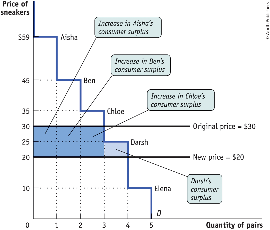
The gain in consumer surplus has two parts:
The dark blue rectangle shows the gain to those who would have bought the sneakers at the original price $30
The light blue rectangle shows the gain to those who wouldn't have bought the good at the original price of $30 but are willing to do so at the new price of $20
Producer surplus
Producer surplus: the difference between the market price and the price at which firms are willing to supply the product
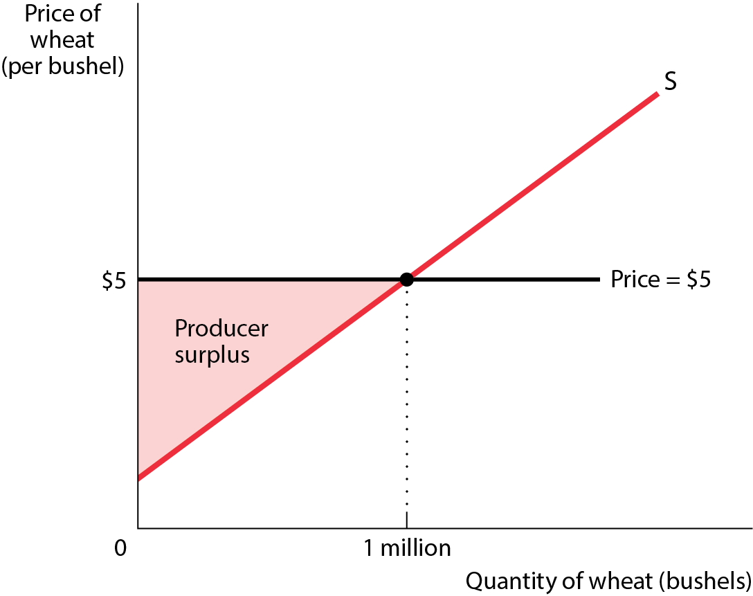
Individual producer surplus: the net gain to an individual seller from selling a good, which is equal to the difference between the price received and the seller’s cost (the seller’s cost includes monetary costs; it may also include other opportunity costs)
Total producer surplus: the sum of individual producer surpluses of all the sellers in a market
Economists use the term producer surplus to refer to both individual and total producer surplus
Producer surplus rises if the price increases
Consumer surplus, producer surplus, and the gains from trade
Total surplus: the sum of the producer and consumer surpluses
The efficiency of markets
Markets are usually efficient: there is no way to make some people better off without making other people worse off
Markets are usually efficient because they maximize total surplus
Three ways you might (successfully) try to increase the total surplus
Reallocate consumption among consumers
Reallocate sales among sellers
Change the quantity traded
Competitive markets are usually efficient:
They allocate consumption of the good to the potential buyers who most value it
They allocate sales to the potential sellers who most value the right to sell the good (e.g., who have the lowest cost)
They ensure that all transactions are mutually beneficial: every consumer who makes a purchase values the good more than every seller who makes a sale
They ensure that no mutually beneficial transactions are missed: every potential buyer who doesn’t make a purchase values the good less than every potential seller who doesn’t make a sale
Three caveats to efficiency
Although a market may be efficient, it isn’t necessarily fair
Markets sometimes fail to deliver efficiency
Even when the market equilibrium maximizes total surplus, this doesn’t mean that it results in the best outcome for every individual consumer or producer
Why reallocating consumption lowers consumer surplus
Everyone who buys a pair of sneakers at the market equilibrium has a willingness to pay of $30 or more, and everyone who doesn’t buy a pair of sneakers has a willingness to pay less than $30
Why reallocating sales lowers producer surplus
Anyone who sells a pair of sneakers at the market equilibrium has a lower cost than anyone who keeps a pair of sneakers
Why changing the quantity lowers the total surplus
Anyone who wouldn’t have bought a pair of sneakers has a willingness to pay of less than $30, and anyone who wouldn’t have sold a pair has a cost of more than $30
Equity and efficiency
Efficiency is important, but society also cares about equity
Sometimes societies choose to have government intervene in markets to increase equity, even though it reduces efficiency
Why markets typically work well
Well-functioning markets are effective because of
Property rights
Economic signals
Why private property matters
Property rights are the rights of owners of valuable items, whether resources or goods, to dispose of those items as they choose
Private property rights create and protect incentives to trade with others and to innovate
Economic signals
An economic signal is any piece of information that helps people make better economic decisions
Prices are the most important signals in a market economy because they convey information about other people’s costs and their willingness to pay
Words of caution
Markets aren’t always efficient; sometimes they fail
When markets are inefficient, opportunities are missed. Some people could be made better off without making other people worse off
When a market is inefficient, we have a market failure
Markets can fail due to market power when a firm has the ability to raise the market price
Markets can fail due to externalities when actions have side effects on the welfare of others
Markets can fail when the nature of the good makes it unsuitable for efficient allocation by a market: public goods, common resources, and private information
Chapter 5: Price Controls and Quotas: Meddling with Markets
What will we learn in this chapter?
What is a market intervention, and why are price controls and quantity controls the two main forms it takes
Why do price and quantity controls create deadweight losses
Who benefits and who loses from market interventions
Why are economists often skeptical of market interventions? And why do governments undertake market interventions even though they create losses to society?
Interference in the market has consequences
Because of rent control policies, an affordable and available rental apartment is hard to find in NYC
Why do governments control prices?
Market prices do not necessarily please buyers or sellers: they may lobby the government to help them by altering the price
Price controls: legal restrictions on how high or low a market price may go. There are two main types
Price ceiling: the maximum price sellers are allowed to charge for a good or service (usually set below the equilibrium)
Price floor: minimum price buyers are required to pay for a good or service (usually set above the equilibrium)
Modeling a price ceiling
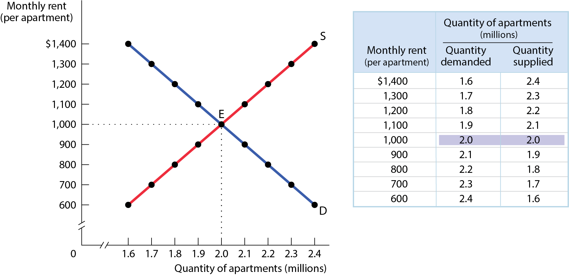
Without government intervention, the market for apartments reached equilibrium at point E with a market rent of $1,000 per month and 2 million apartments rented
This price ceiling creates a persistent shortage of 400,000 units: 400,000 households who want apartments at the legal rent of $800 but can’t get them
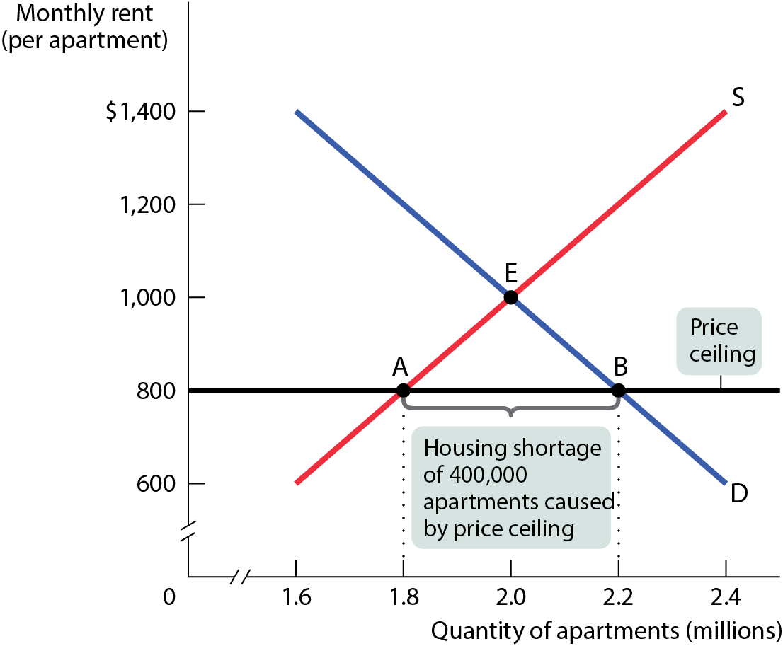
How price ceilings cause inefficiency
Price ceilings cause predictable side effects:
Inefficiently low quantity
Inefficient allocation to customers
Wasted resources
Inefficiently low quality
Black markets
Inefficiently low quantity graphed
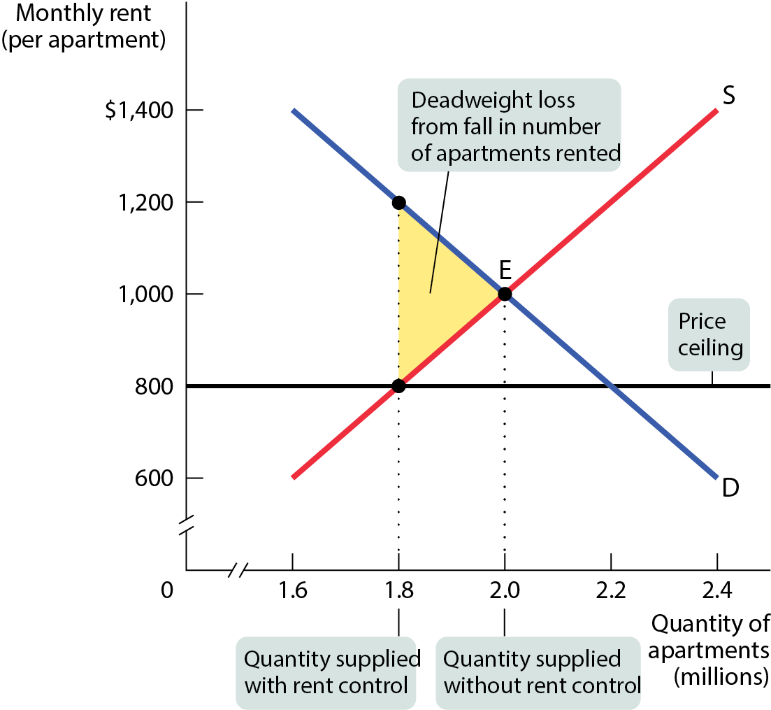
The area of the shaded triangle corresponds to the amount of total surplus lost due to the inefficient low quantity transacted
Inefficient allocation to customers
Price controls lead to misallocation of apartments: people who badly need a place to live may not find out, but some apartments may be occupied by people with much less urgent needs
Under rent control, people usually get apartments through luck or personal connections
Wasted resources
People expend money, effort, and time to cope with shortages caused by the price ceiling
Back in 1979, U.S price controls on gasoline led to shortages that forced millions of Americans to wait in line at gas stations for hours each week
The opportunity cost of the time spent in line - the wages not earned, the leisure time not enjoyed – constituted wasted resources
Rent control creates missed opportunities
Inefficicently low quality
At the controlled price, sellers have more customers than goods
In a free market, this would be an opportunity to profit by raising prices
But when prices are controlled, sellers can’t raise prices
Sellers respond to this problem in two ways
Reduce quality
Reduce service
Landlords of rent-controlled housing have no incentive to provide better conditions
Shadow markets
A shadow market is a market in which goods or services are bought and sold illegally, either because they are prohibited or because the equilibrium price is illegal
Some tenants are willing to bribe landlords
Shadow markets encourage disrespect for the law in general and worsen the position of those who are honest
Shadow markets can diminish some of the inefficiencies, but in the end, society as a whole is worse
So why are there price ceilings
They do benefit some people (who are typically better organized and more vocal than those who are harmed by them)
If the price ceiling has been in effect for a long time, buyers may not have a realistic idea of what would happen without it
Government officials often do not understand supply and demand analysis
Venezuela's food shortages show how price controls disproportionately hurt the people they were signed to benefit
Price floors
Sometimes governments intervene to push market prices up instead of down
The generous minimum wage in many European countries has contributed to a high rate of unemployment and the flourishing of an illegal labor market
Modeling a price floor
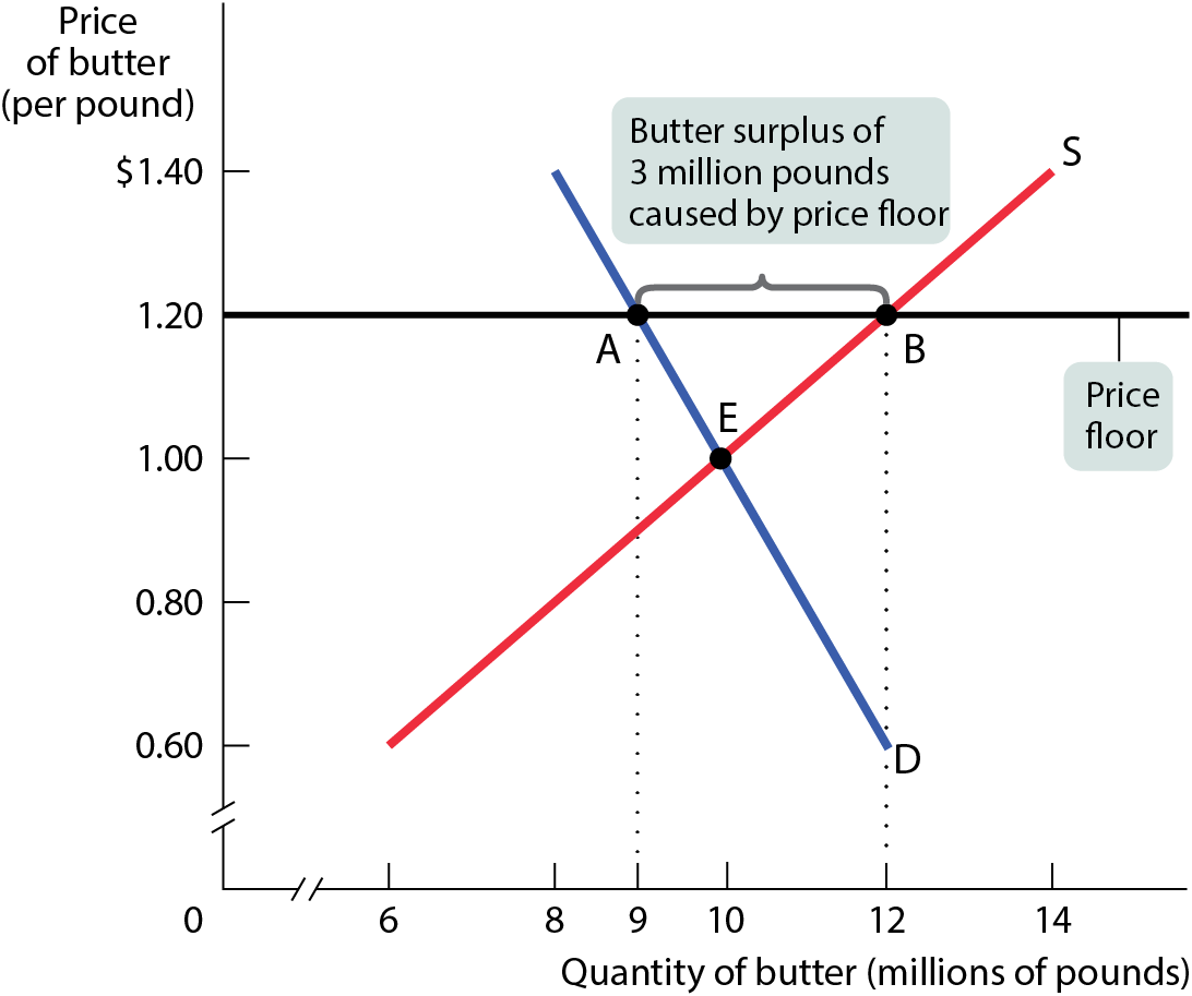
The quantity of butter demanded falls to 9 million pounds, and the quantity supplied rises to 12 million pounds, generating a persistent surplus of 3 million pounds of butter
How a price floor causes inefficiency
Price floors cause predictable side effects:
Deadweight loss
Inefficient allocation of sales among sellers
Waste of resources
Inefficiency in high-quality
Temptation to break the law by selling below the legal price
Inefficiently low quality
A price floor reduces the quantity demanded below the market equilibrium quantity and leads to a deadweight loss
Inefficient allocation of sales among sellers
Price floors can lead to Inefficient allocation of sales among sellers
Sellers who are willing to sell at the lowest price are unable to make sales
Sales go to the sellers who are only willing to sell at a higher price
An example is the two-tier labor market found in many European countries
A high minimum wage led to a two-tiered system, composed of the fortunate who had good jobs in the formal market and the rest who were locked out without any prospect of finding a good job
Wasted resources: price floors
Price floor encourages waste
To deal with the surplus generated by agricultural price floors, the U.S government sometimes buys back the excess and donates or destroys it
Inefficiently high quality
Price floors encouraged sellers to offer goods of inefficiently high quality – the quality that is higher than buyers are willing to pay for
When transatlantic airfares were set by international treaty, airlines could not offer lower prices, so they offered expensive services instead. Most flyers, however, would prefer lower airfares and less food
Illegal activity
Price floors encourage shadow markets
There are willing sellers (and buyers) at illegal prices, so they are tempted to break the law and trade with each other
So why are there price floors
Same as price ceilings
They do benefit some people (who are typically better organized and more vocal than those who are harmed by them)
Government officials often do not understand supply and demand analysis
Controlling quantities
Governments sometimes control quantity instead of price
quota: an upper limit, set by the government, on the quantity of some good that can be bought or sold; also referred to as a quantity control
Quota limit: the total amount of a good under a quota or quantity control that can be legally transacted
License: the right, conferred by the government, to supply a good
Effect of a quota on the market for taxi rides
Demand price: the price of a given quantity at which consumers will demand that quantity
Supply price: the price fo a given quantity at which producers will supply that quantity
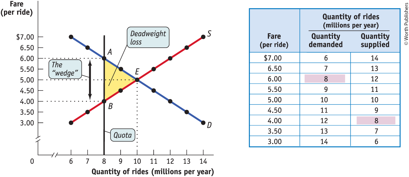
The wedge or quota rent is the difference between the demand price and the supply price at the quota limit, equal to the market price of the license when the license is traded
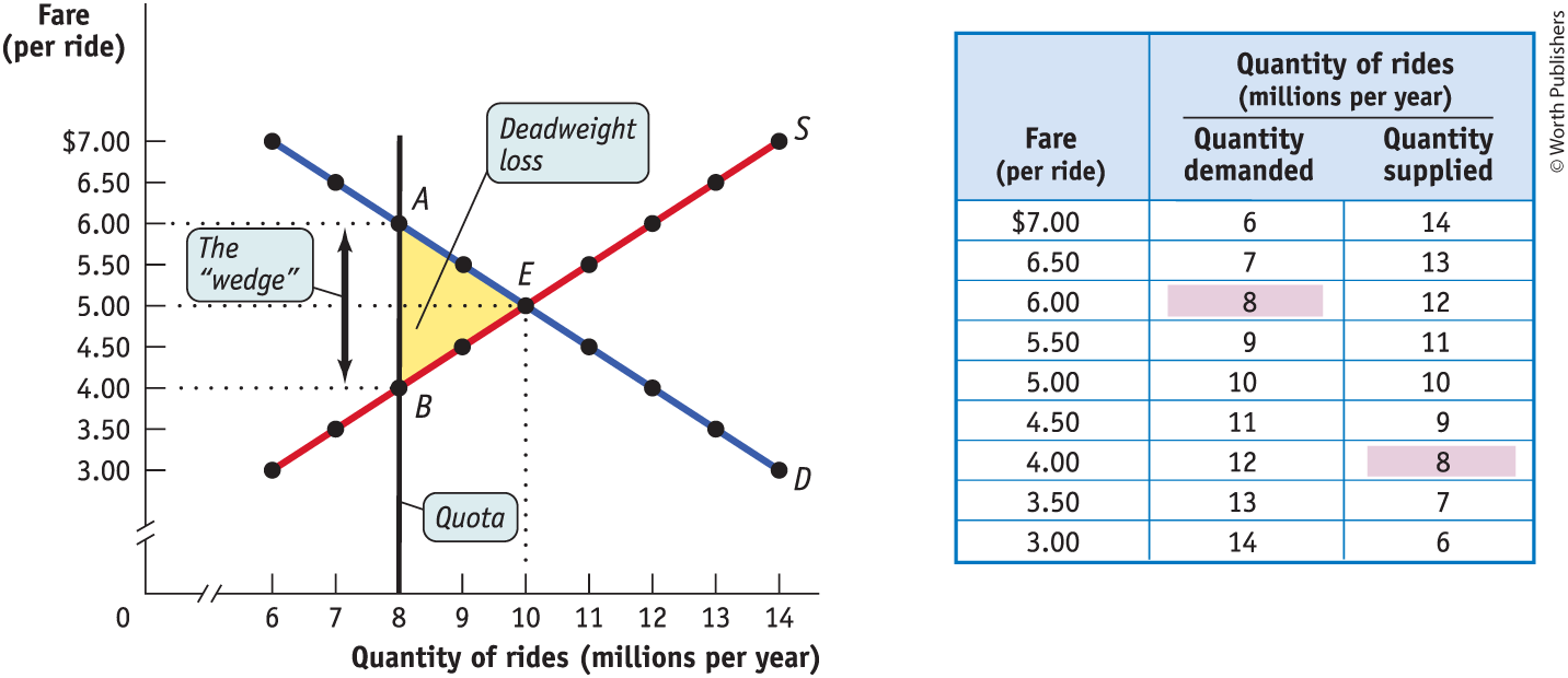
The costs of quantity controls
Like price controls, quotas impose losses on society
Deadweight loss (some mutually beneficial transactions don’t occur)
Incentives for illegal activities
Unlicensed cabs are a side effect of quantity controls… but also an opportunity for alternate models like Uber
Chapter 6: Elasticity
What will we learn in this chapter?
Why is elasticity used to measure the response to changes in prices or income?
What are the different elasticity measures, and what do they mean
What factors influence the size of these various elasticities
Why is it vitally important to determine the size of the relevant elasticity before setting prices or government fees
Price elasticity of demand
Price elasticity of demand is the measure of price responsiveness
A demand is elastic when an increase in price reduces the quantity demanded a lot
A demand is inelastic when an increase in price reduces quantity demanded just a little
Calculating the price elasticity of demand
Price elasticity of demand = % change in quantity demanded / % change in price
The midpoint method
There is a problem: our percent change calculation depends on our choice of starting point
Ex. gasoline costs three times as much per gallon in Europe as it does in the United States. What is the percent difference between American and European gas prices? It depends on which way you measure it
European prices are 200% higher
American prices are 66.67% lower
To solve, we calculate the price elasticity of demand using the midpoint formula for percentage changes
% change in X = (change in X/Avg value of X) x 100
Avg value of X =(starting value of X + final value of X)/2
Estimating elasticities
Economists are interested in the price elasticity of demand
Estimating elasticity is crucial to understanding and predicting market outcomes
Inelastic
Gasoline
College (in-state)
Airline travel (business)
Soda
Elastic
Housing
College (out of state)
Airline travel (leisure)
Coke/Pepsi
Interpreting the price elasticity of demand
Classification of price elasticity of demand:
A good can have a price elasticity as low as zero, as high as infinity
If a price elasticity <1, the demand curve is inelastic
If a price elasticity >1, the demand curve is elastic
If a price elasticity = 1, the demand curve is unit-elastic
Elasticity and total revenue
Total revenue: price times quantity sold
TR = P x Q
Sellers need to know how elastic demand is so they can plan
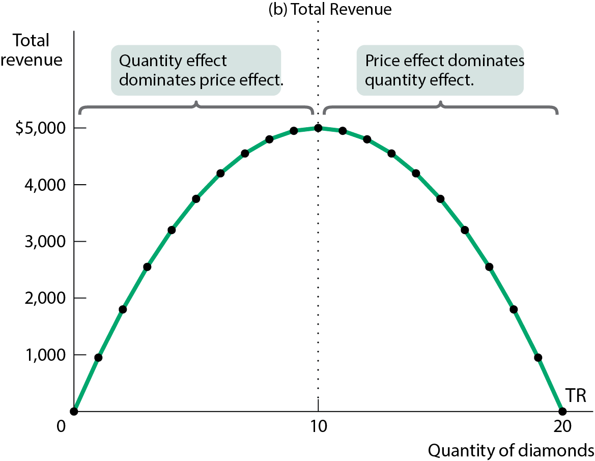
When demand is inelastic, the price effect dominates the quantity effect
So an increase in price will cause only a slight reduction in the quantity demanded
In this instance, total revenue will rise when the price rises
When demand is elastic, the quantity effect dominates the price effect
So an increase in price will cause a significant reduction in the quantity demanded
In this instance, total revenue will fall when the price rises
When demand is unit-elastic, the quantity effect equals the price effect
So an increase in price exactly balances the reduction in the quantity demanded
In this instance, total revenue does not change
Price effect and quantity effect
When a seller raises the price of a good, there are two countervailing effects
A price effect: after a price increase, each unit sells at a higher price, which tends to raise revenue
A quantity effect: after a price increase, fewer units are sold, which tends to lower revenue
What factors determine the price elasticity of demand
Whether the good is a necessity or a luxury
For necessities, quantity demanded does not change much in response to a change in P
For luxuries, the quantity demanded is more sensitive to a change in price
The availability of close substitutes
Fewer substitutes make it harder for consumers to adjust Q when P changes, so demand is inelastic
Many substitutes make it easier for consumers to switch brands when prices change, so demand is elastic
The share of income spent on the good
It feels cheaper when we spend a smaller share of our income on the good
It feels more expensive when we spend a greater share of our income on the good
Time elapsed since the price change
Less time to adjust means lower elasticity
Over time, consumers can adjust their behavior by finding substitutes (making demand more elastic)
Applications of elasticity of demand
Why the war on drugs is hard to win
Because demand for most illegal drugs is inelastic, drug dealers earn greater revenue and gain more power as the war on drugs reduces the supply
Other demand elasticities
The cross-price elasticity of demand measures how sensitive the quantity demanded of good A is to the price of good B
Cross price elasticity of demand = % change in quantity of A demanded/ % change in price of B
Cross-price elasticity of demand
For substitutes, the cross-price elasticity of demand is positive
An increase in the price of one brand of cookies will increase the demand for other brands
The size of the cross-price elasticity shows how closely substitutable the two goods are
For complements, the cross-price elasticity of demand is negative
An increase in the price of milk causes a decrease in demand for oreos
The size of the cross-price elasticity shows how closely complementary the two goods are
Income elasticity of demand
The income elasticity of demand measures how sensitive the quantity demanded of a good is to changes in income
Income elasticity of demand = % change in quantity demanded/ % change in income
The income elasticity of demand can be used to distinguish normal from inferior goods
For normal goods, income elasticity is positive
For inferior goods, income elasticity is negative
Normal goods can be income-elastic or not
For income-elastic goods, income elasticity is greater than 1
For income-inelastic goods, income elasticity is positive but less than 1
Measuring the price elasticity of supply
Usually, sellers offer more when prices are higher, but how strong is that relationship
Similar to the price elasticity of demand
Price elasticity of supply = % change in quantity supplied/ % change in price
Elasticity of supply
The supply curve is elastic if a rise in price increases the quantity supplied a lot
The supply curve is inelastic if a rise in price increases the quantity supplied just a little
What factors determine the price elasticity of supply
Availability of inputs
If an increase in production is very expensive (inputs are not easily available or can’t be shifted), then supply will be inelastic
If production can be increased cheaply, then the supply will be elastic
Time
Price elasticity of supply increases as producers have more time to respond to price changes changes
The long-run price elasticity of supply is usually higher than the short-run elasticity
Chapter 7: Taxes
What will we learn in this chapter?
How do taxes affect supply and demand
What factors determine who bears the burden of a tax
What are the costs and benefits of a tax, and why is the cost greater than the tax revenue generated
What is the difference between progressive and regressive taxes
Why is there a trade-off between equity and efficiency in the design of a tax system
How is the U.S. tax system structured
The effect of an excise tax on quantities and prices
Taxes drive a wedge between the price buyers pay and the price sellers receive
To analyze the effects, we’ll graph two scenarios
When the tax is levied on sellers
When the tax is levied on buyers
The incidence of a tax is a measure of who really pays it
An excise tax imposed on hotel owners
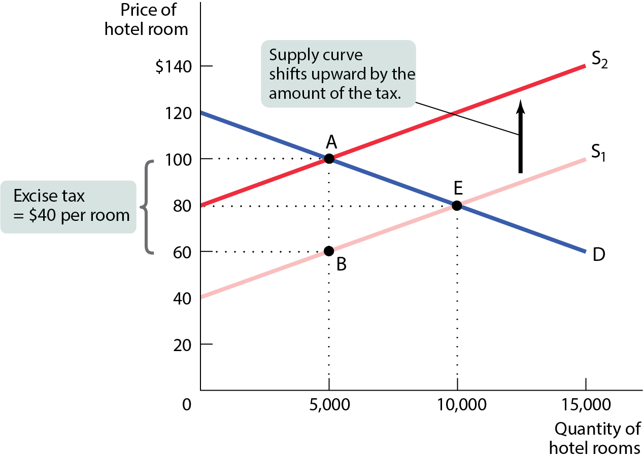
The $40 excise tax (a tax charged on each unit sold) is shared between buyers and sellers
The equilibrium price of hotel rooms rises to $100 a night
Hotel guests bear some of the burden as the price rises from $80 to $100
Hotel owners also bear some of the burden as their price (net of the tax paid) falls from $80 to $60
An excise tax imposed on hotel guests
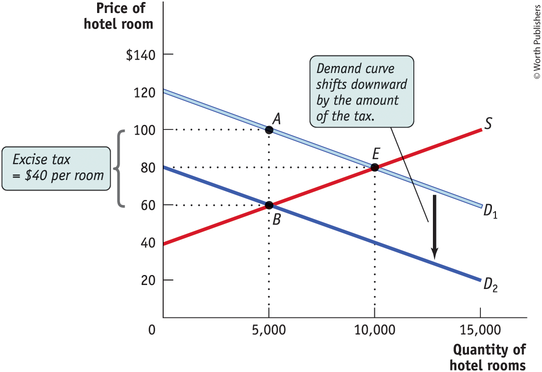
The $40 excise tax is shared between buyers and sellers
The equilibrium price of hotel rooms falls to $60 a night
Hotel guests bear some of the burden as the price paid by the guests (price plus tax) rises from $80 to $100
Hotel owners also bear some of the burden as their price falls from $80 to $60
The incidence of an excise tax doesn’t depend on who officially pays the tax
Price elasticities and tax incidence
Although both buyer and seller share the burden of the tax, it’s not necessarily an equal burden
In a long-distance relationship, for example, who will do more of the driving
Does the “tax” fall more heavily on the more committed partner
When an excise tax is paid mainly by consumers
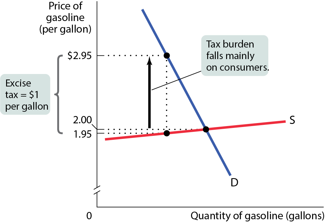
When the price elasticity of demand is low and the price elasticity of supply is high, the burden of an excise tax falls mainly on consumers
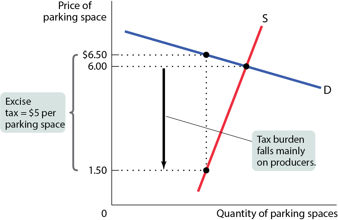
When an excise tax is paid mainly by producers
When the price elasticity of demand is high and the price elasticity of supply is low, the burden of an excise tax falls mainly on producers
The revenue from an excise tax
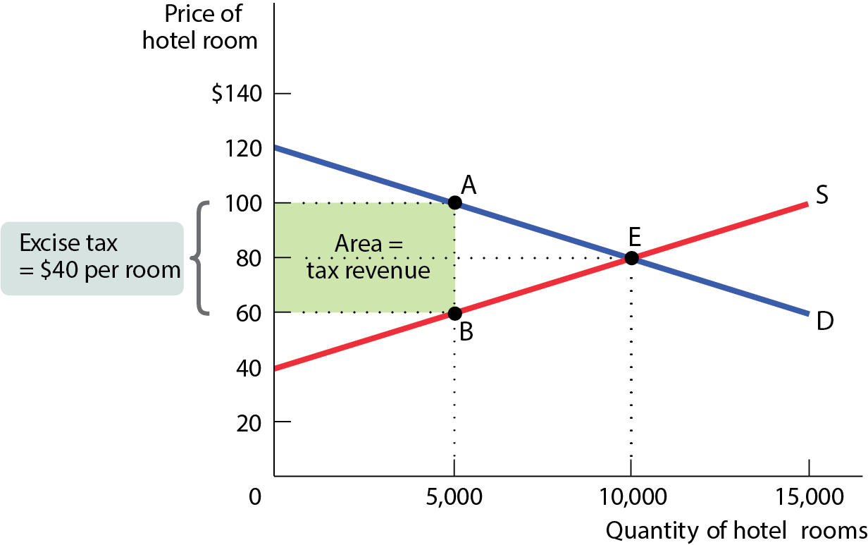
The tax revenue collected = height x width
$40 per room x 5000 rooms =$ 200,000
Increasing the tax rate does not necessarily increase revenue
On the one hand, the tax increase means the government raises more revenue per unit sold, thereby increasing total tax revenue.
On the other hand, it reduces the quantity of sales, which decreases tax revenue
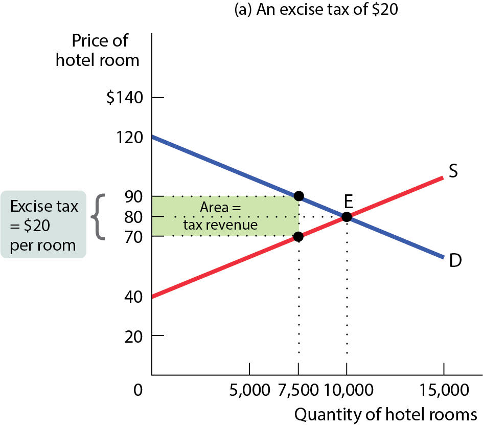
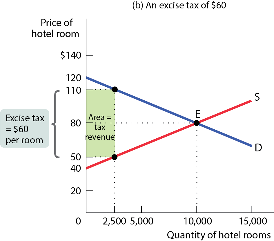
If the price elasticities of both supply and demand are low, the tax increase won’t reduce the quantity of the good sold very much, so tax revenue will definitely rise
If the price elasticities are high enough, the tax reduces the quantity sold so much so that tax revenue falls
If the price elasticities are high, the result is less certain and dependent on how much lower the initial tax rate was
The cost of taxation
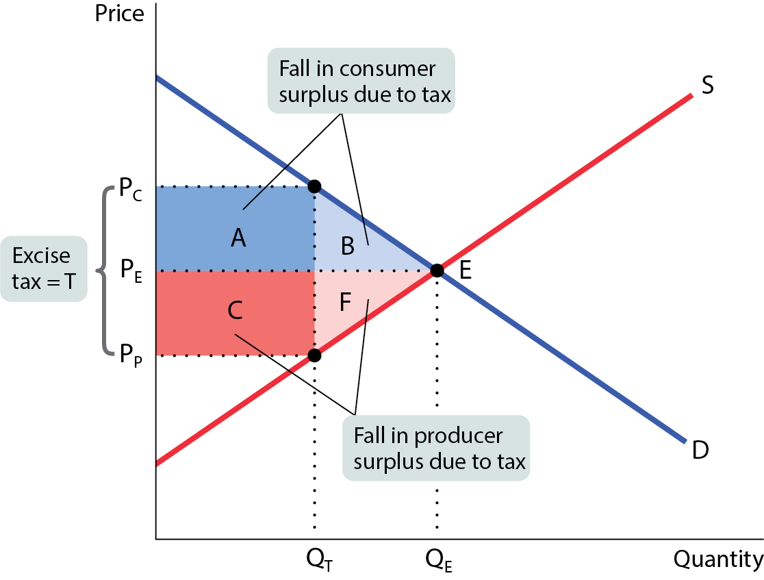
An excise tax imposes costs because it prevents mutually beneficial transactions (Qe - Qt)
The value of such transactions is called the deadweight loss (areas B and F)
A tax generates revenue and creates a deadweight loss
There are also costs not shown in: the administrative costs of a tax are the resources used for its collection, for the method of payment, and for any attempts to evade the tax
Taxes cost society time and effort that could have been used elsewhere
Total inefficiency of tax = deadweight loss + administrative costs
Elastics and deadweight loss
The greater the price elasticity of demand or supply, the greater the tax-induced fall in the quantity transacted
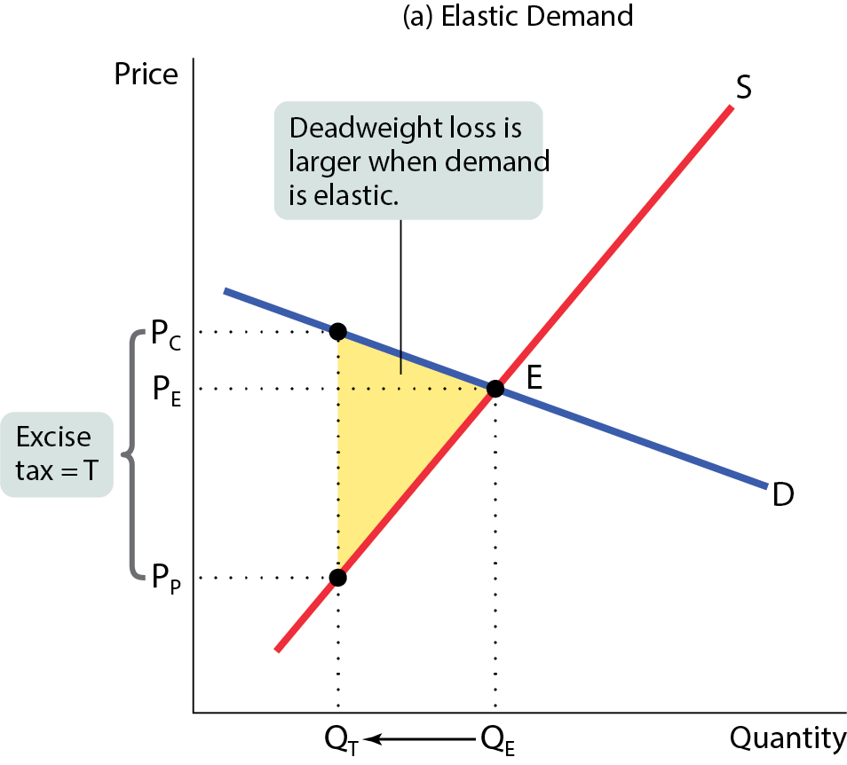
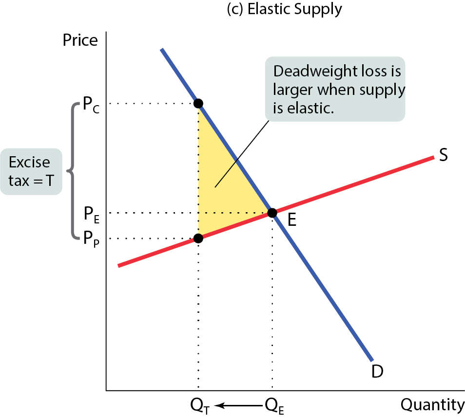
The lower the price elasticity of demand or supply, the smaller the tax-induced fall in the quantity transacted, and the smaller the dead loss
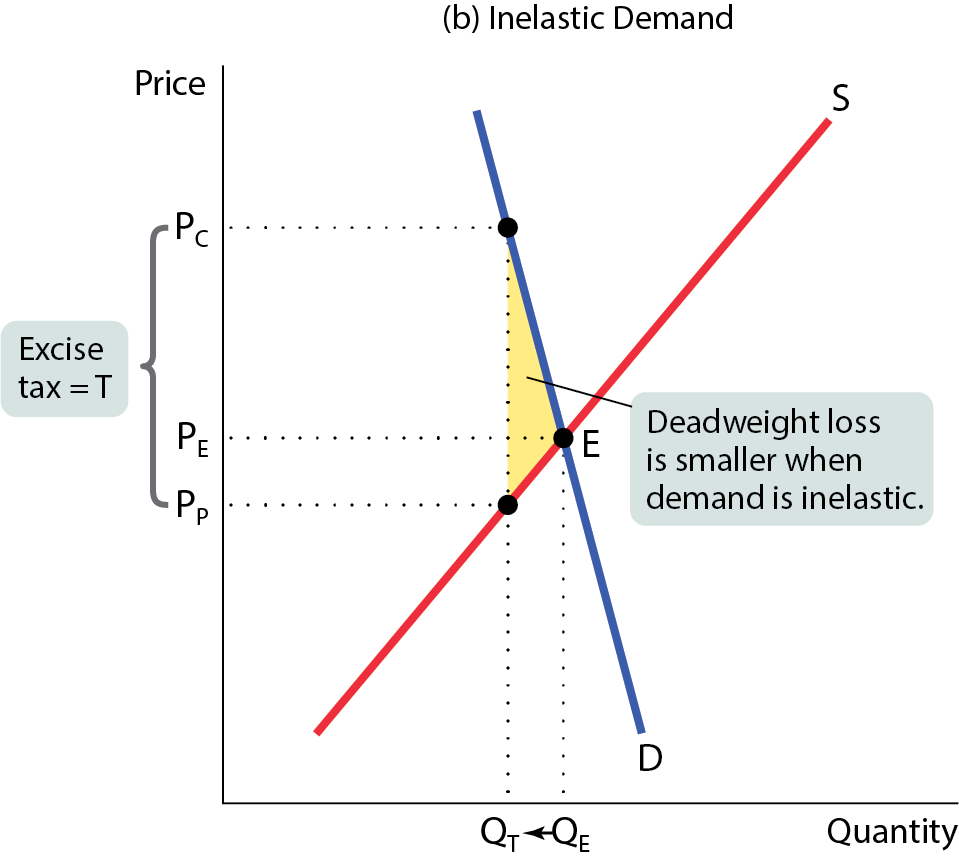
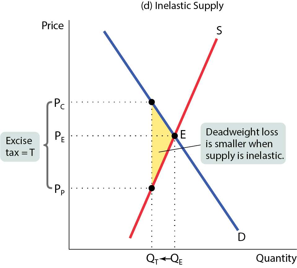
If the goal in tax policy is efficiency (minimizing deadweight loss), then policymakers should choose the goods with the lowest price elasticities
A tax on insulin would be efficient - but not necessarily fair
Tax fairness and tax efficiency
The two principles of tax fairness
The benefits principle: those who benefit from public spending should bear the burden of the tax that pays for that spending
Ex. Those who use a road should pay for that road’s upkeep
The ability-to-pay principle: those with greater ability to pay a tax should pay more
Ex. Whiskey Rebellion of 1791, there was a protest against the fact that small distillers paid a higher share of their income than large distillers
There is usually a trade-off between equity and efficiency: the system can be made more efficient only by making it less fair, and vice versa
Understanding the tax system
The tax base is the measure, such as income or property value, that determines how much tax an individual or firm pays
Income tax depends on income from wages and investments
Payroll tax depends on the earnings that an employer pays an employee
Sales tax depends on the value of goods sold
Profit tax depends on a firm's profit
Property tax depends on the value of the property, such as a home
Wealth tax is a tax that depends on an individual's wealth
The tax structure specifies how the tax depends on the tax base
A progressive tax takes a larger share of the income of high-income taxpayers than that of low-income taxpayers
A regressive tax takes a smaller share of the income of high-income taxpayers than that of low-income taxpayers
The marginal tax rate is the percentage of an increase in income that is taxed away
Taxes in the United States
Tax competition: A state or local government that imposes high taxes on people with high incomes faces the prospect that those people may move to other locations where taxes are lower
Chapter 9: Decision making
What will we learn in this chapter?
Why does good decision-making depend on accurately defining costs and benefits?
What is the difference between explicit and implicit costs?
What is the difference between accounting profit and economic profit, and why is the economic profit the correct basis for decisions?
What are three types of economic decisions?
Why do people behave in irrational yet predictable ways sometimes?
Why are decisions involving time different, and how should they be made?
Costs, benefits, and profits
Our decisions depend on comparing costs with benefits
Recall opportunity costs
Because resources are scarce, the true cost of anything is what you must give up to get it
Explicit V. implicit costs
An explicit cost is a cost that requires an outlay of money
Ex. another year in school includes tuition
An implicit cost does not require an outlay of money; it is measured by the value, in dollar terms, of benefits that are forgone
Ex. wages are forgone because of being a full-time student
Opportunity cost = total explicit cost + total implicit cost
Accounting V. economic profit
Accounting profit = revenue - explicit cost
Economic profit = revenue - opportunity cost (of all resources used)
= revenue - (explicit cost + implicit cost)
Economics profit
Less than accounting profit
Show a more complete picture of costs
Helps businesses and individuals make better-informed decisions
Is the measure economists use
Math concepts
Average =
Marginal = change in total/change in input
The implicit costs of capital
Capital is the total value of assets owned by an individual or a firm - physical assets plus financial assets
The implicit cost of capital is the opportunity cost of the use of one’s own capital; that is, the income earned if the capital had been employed in its next best alternative use
Ex. forgone interest income
How many V. either-or decisions
There are two different types of decisions
A choice between two alternatives (either-or)
A more complex choice that requires us to choose at the margin (how much)
Making an either-or decision
Principle of either-or decision-making
When faced with an either-or choice between two activities (all else equal), choose the one with the positive economic profit
Pitfall
If there are three or more options, the either-or principle still applies
Making “how much” decisions: the role of marginal analysis
How much is a decision at the margin
Marginal analysis: comparing the benefit of doing a little bit more of something with the cost of doing a little bit more of something – comparing marginal benefit with marginal cost
Marginal cost of producing a good or service is the additional cost incurred by producing one more unit of that good or service
Marginal cost
The marginal cost curve shows how the cost of producing one more unit depends on the quantity that has already been produced
Each product has a unique marginal cost. Some basic shapes
Increasing marginal cost: each additional unit costs more to produce than the previous one
Ex. because of paying costly overtime wages
Constant marginal cost: each additional unit costs the same to produce as the previous one
Ex. the cost of growing one more plant is the same regardless of how many plants have been produced
Decreasing marginal cost: each additional unit costs less to produce than the previous one
Often, due to learning effects in production, when workers gain skills and experience
Pitfalls
Marginal costs and total costs don’t always move in the same direction
Ex. if the marginal cost of producing the first widget is $5, the second $4, and the third $3, the total cost rises as the marginal cost falls
Marginal benefits
Marginal benefit: the additional benefit derived from producing one more unit of a good or service
There is a decreasing marginal benefit from an activity when each additional unit of the activity yields less benefit than the previous unit
The marginal benefit curve shows how the benefit from producing one more unit depends on the quantity that has already been produced
Marginal analysis
Optimal quantity: the quantity that generates the highest possible total profit
Profit-maximizing of marginal analysis: the largest quantity at which the marginal benefit is greater than or equal to the marginal cost
Pit falls
You're trying to maximize the difference between benefits and costs
What we're doing is setting marginal (not total) benefit and cost equal to each other
Only when marginal benefit and marginal costs are equal, the difference between total benefit and total cost is at a maximum
Sunk costs
Sunk cost: a cost that has already been incurred and is not recoverable
A sunk cost should be ignored in decisions about future actions (but this is sometimes hard to do)
Ex. if you lose your concert ticket, the $80 you’ve already spent on them is irrelevant to the decision whether to replace them – it is a sunk cost
Reasons people might rationally choose a worse payoff
Concerns about fairness: providing for others sometimes trumps self-interest
Nonmonetary rewards: experiences that feel good, such as travel, quality time spent with family and friends, playing a sport, etc.
Bounded rationality: making a choice that is close to but not exactly the one that gives you the best payoff – the good enough method of decision-making. Choosing the best option requires mental effort, and if it’s too costly, it might make sense to choose a good enough option
Risk aversion: willingness to sacrifice some economic payoff in order to avoid a potential loss. Because risk makes most people uncomfortable, they give up some potential gain to avoid risk
Irrationality: an economist’s view
An irrational decision maker chooses an option that leaves them worse off than choosing another available option that would have left them better off
8 common decision-making mistakes -
Misperceptions of opportunity costs
People tend to ignore opportunity costs when they are nonmonetary
Another misconception is believing that a sunk cost is an opportunity cost
Over confidence
We tend to think we know more than we actually do
Unrealistic expectations
Most of us are overly optimistic about our future behavior and level of discipline
Counting dollars unequally
Mental accounting: the habit of mentally assigning dollars to different accounts so that some dollars are worth more than others
Loss aversion
An over-sensitivity to loss that leads to an unwillingness to recognize a loss and move on
Framing bias
The tendency to make decisions based on how the choices are presented
Ex. shoppers perceive $0.99 as more attractive than $1
Fomo
The tendency to invest in an asset based on past performance, arising from the fear that one is a “loser,” doesn't make a big profit like earlier investors
Ex. people who missed out on buying Bitcoin early on are buying it now
Status quo bias
The tendency to avoid making a decision altogether
Ex. if a company has an automatic enrollment in a 401(k) program with an opt-out option, people tend not to opt out and go with the status quo
Rational models of irrational people
Why do economists still use models based on rational behavior when people are at times irrational?
Rational models still provide robust predictions about how people behave
Ex. we buy less when prices rise, which is rational behavior
Market forces compel people to behave more rationally over time. When people are disciplined for their mistakes, rationality will win out over time
It makes modeling simpler. Remember that models are built on generalizations, and it’s much harder to extrapolate from messy, irrational behavior
Midterm 1 ↑
Chapter 13: The Rational Consumer
What will we learn in this chapter?
What factors determine how consumers spend their income
Why do economists use the concept of utility to describe people's tastes
Why does the principle of diminishing marginal utility accurately describe consumer behavior
What is the optimal consumption bundle, and why do we use marginal analysis to determine it?
How do income and substitution effects show the effects of changes in income and prices on consumers' choices?
Utility and consumption
We suppose that each individual is trying to maximize the satisfaction gained from consumption
Utility is the value or satisfaction from consumption
An individual's consumption bundle is the collection of all the goods and services consumed by that individual
An individual's utility function gives the total utility generated by their consumption bundle
Util is a unit of utility
Marginal utility (MU) is the change in utility from consuming an additional unit
Diminishing marginal utility is the fact that each additional unit of a good adds less to utility than the previous unit
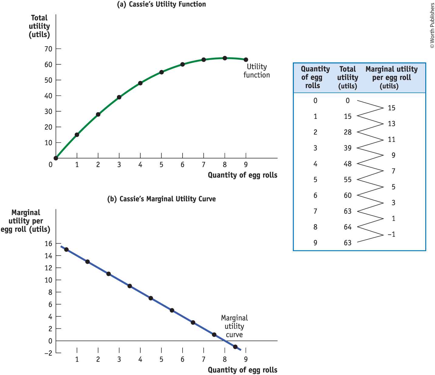
Cassie's total utility and marginal utility
Each additional egg roll gives Cassie less additional utility than the previous egg roll
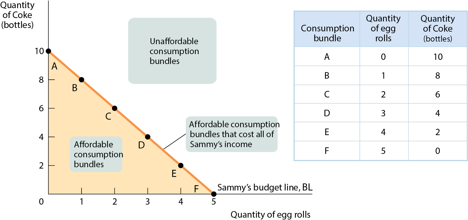
Graphing the budget line
Sam has a weekly income of $20; he spends all of it on egg rolls and Coke. Egg rolls cost $4 per roll, and Coke costs $2 per bottle
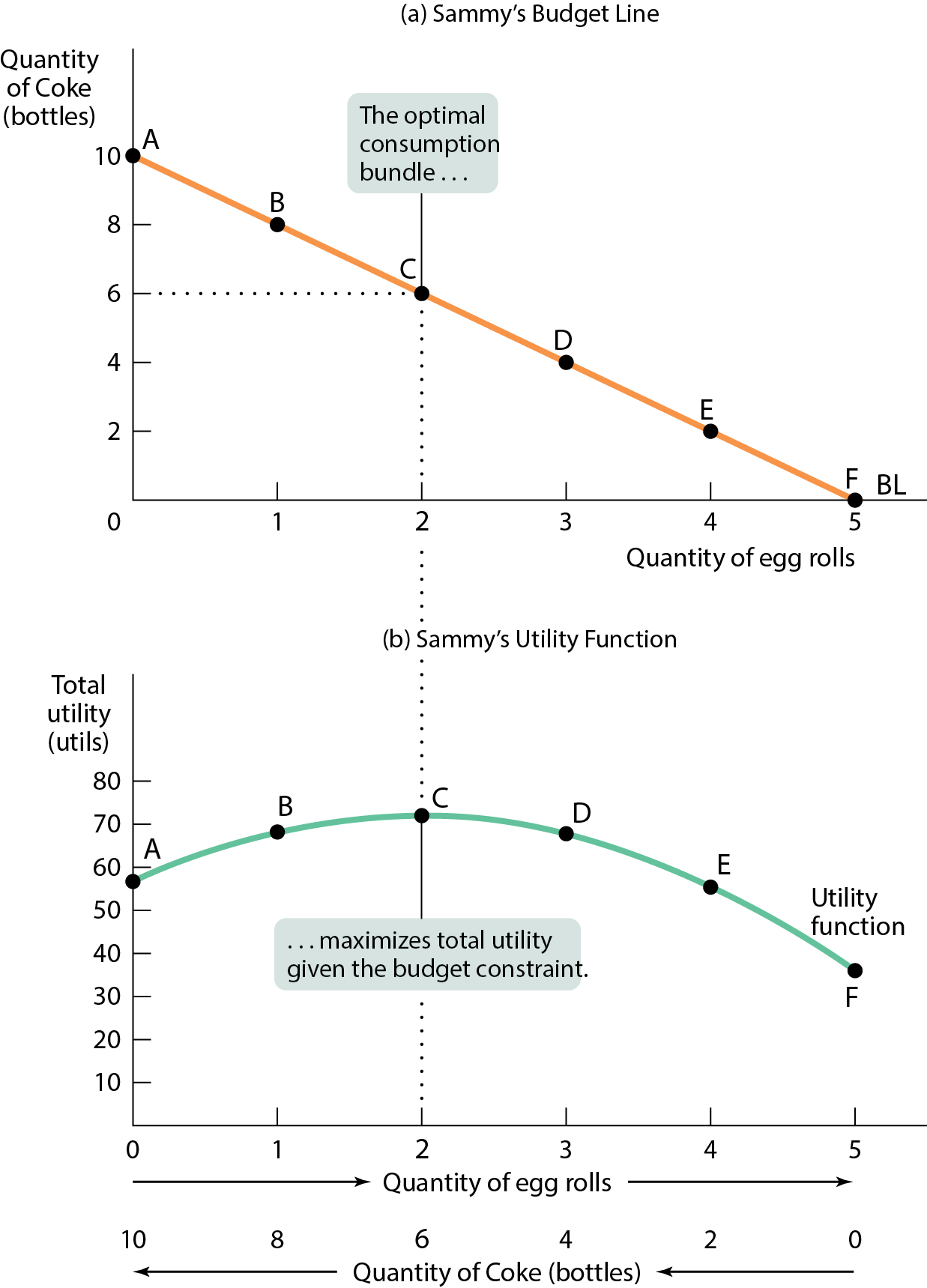
Optimal consumption
Table 2: Sam’s Budget and Total Utility
Consumption bundle | Quantity of egg rolls | Utility from egg rolls (utils) | Quantity of Coke (bottles) | Utility from Cokes (utils) | Total utility (utils) |
|---|---|---|---|---|---|
A | 0 | 0 | 10 | 56.7 | 56.7 |
B | 1 | 15 | 8 | 53.2 | 68.2 |
C | 2 | 25 | 6 | 47.0 | 72.0 |
D | 3 | 31 | 4 | 36.8 | 67.8 |
E | 4 | 34 | 2 | 21.4 | 55.4 |
F | 5 | 36 | 0 | 0 | 36.0 |
The optimal consumption bundle is the one that maximizes a consumer's total utility given their budget constraint
Spending the marginal dollar
We can find the optimal consumption choice by choosing the bundle at which total utility is maximized
But we can use marginal analysis instead, turning it into a how much problem
We ask if the consumer can make themselves better off by spending a little bit more on either good
To answer this question, we must calculate the marginal utility per dollar
Marginal utility per dollar
Marginal utility is the additional utility a consumer gets from consuming one or more units of a good or service
The marginal utility per dollar spent on a good or service is the additional utility from spending one more dollar on that good or service
To find the marginal utility per dollar, we must divide the marginal utility of the good by its price
Marginal utility per dollar declines as the quantity of that good consumed rises, due to diminishing marginal utility
Comparing marginal utility
The general rule: compare the MU and the price for all goods, and then adjust your spending toward the goods that give you more marginal utility per dollar
Adjusting toward the optimal bundle
Optimal consumption bundle is always where MU/P (a) = MU/P (b)
If the marginal utility per dollar is higher for A than for B, buying more of A and less of B would increase the total utility
If marginal utility per dollar on B is higher, increase utility by spending less on A and more on B
Utility maximizing principle of marginal analysis
Utility-maximizing principle of marginal analysis: When a consumer maximizes utility in the face of a budget constraint, the marginal utility per dollar spent on each good or service in the consumption bundle is the same
If the price rises, the marginal utility per dollar spent on the good falls, and the consumer can increase their utility by buying less of this good and more of other goods
Pitfalls
The right marginal comparison:
Production decisions set the marginal benefit of some activity equal to its marginal cost
Consumption decisions set the marginal utility per dollar equal for each good
Unlike producers, consumers face budget constraints. Consuming more of one good requires consuming less of another
The right marginal decisions set the marginal utility per dollar equal for each good. Only then is there no way to rearrange consumption and get more utility from one's budget
The demand curve and substitution effect
The substitution effect (of a change in price) is the change in the quantity consumed of that good as the consumer substitutes the good that has become relatively cheaper for the good that has become relatively more expensive
Demand curve and income effect
The income effect (change in price) is the change in the quantity consumed of a good that results from a change in the consumer’s purchasing power due to the change in the price of a good
A change in the price of a good effectively changes a consumer's income
For most goods, the income effect has no significant effect on consumption. Most market demand curves slope downward because of the substitution effect
When it matters at all, the income effect reinforces the substitution effect
Giffen goods
In the case of an inferior good, the income and substitution effects work in opposite directions
Giffen good: a very rare inferior good for which the income effect outweighs the substitution effect, and the demand curve slopes upward
Chapter 14: Behind the supply curve
What will we learn in this chapter?
What is a firm's production function
Why is production often subject to diminishing returns to inputs
What types of costs does a firm face, and how does the firm generate its marginal and average cost curves
Why do a firm's costs differ in the short run and in the long run
What is increasing returns to scale, and what advantages does it give
The production function
A firm is an organization that produces goods or services for sale
Production is the process of turning inputs into outputs
A production function is the relationship between the quantity of inputs a firm uses and the quantity of output it produces
A fixed input is an input whose quantity is fixed for a period of time and cannot be varied
Variable input is an input whose quantity the firm can vary at any time
Inputs and output
The long run is the period in which all inputs can be varied
The short run is the period in which at least one input is fixed
The total product curve shows how the quantity of output depends on the quantity of the variable input for a given quantity of the fixed input
Production function and total product curve
The curve slopes upward because more wheat is produced as more workers are employed. It becomes flatter because the marginal product of labor declines as more workers are employed
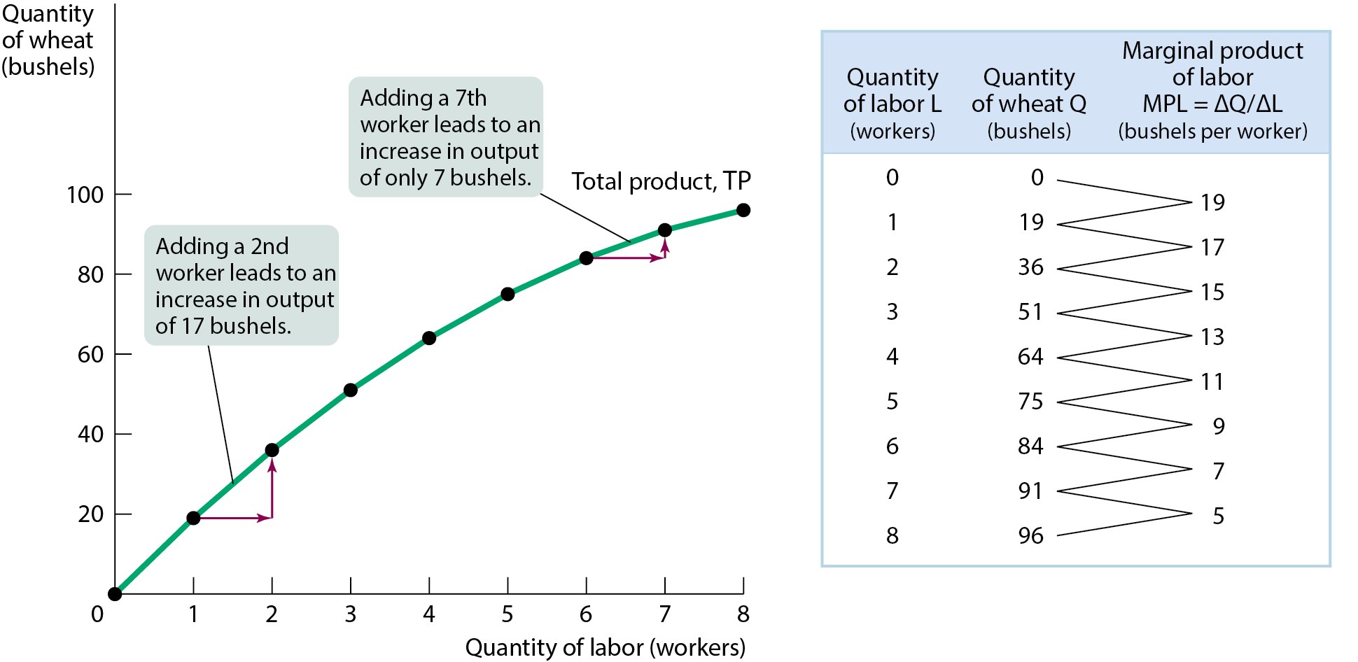
The marginal product of an input is the additional quantity of output that is produced by using one or more units of that input
Marginal product of labor(MPL) is the change in output resulting from a one-unit increase in the amount of labor input
MPL equals the slope of the total product curve
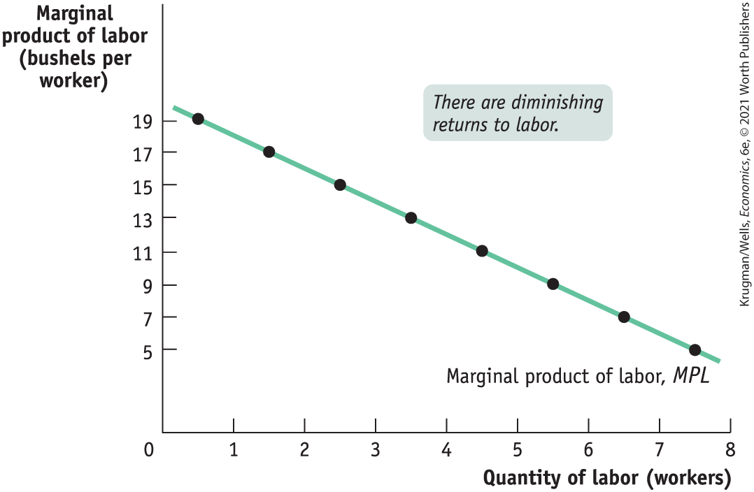
In Figure 1, MPL declines as more workers are hired. As employment increases, the total product curve gets flatter
Figure 2 shows how MPL depends on the number of workers
Diminishing returns to an input
diminishing returns to an input: an increase in the quantity of that input, holding the levels of all other inputs fixed, reduces that input's marginal product
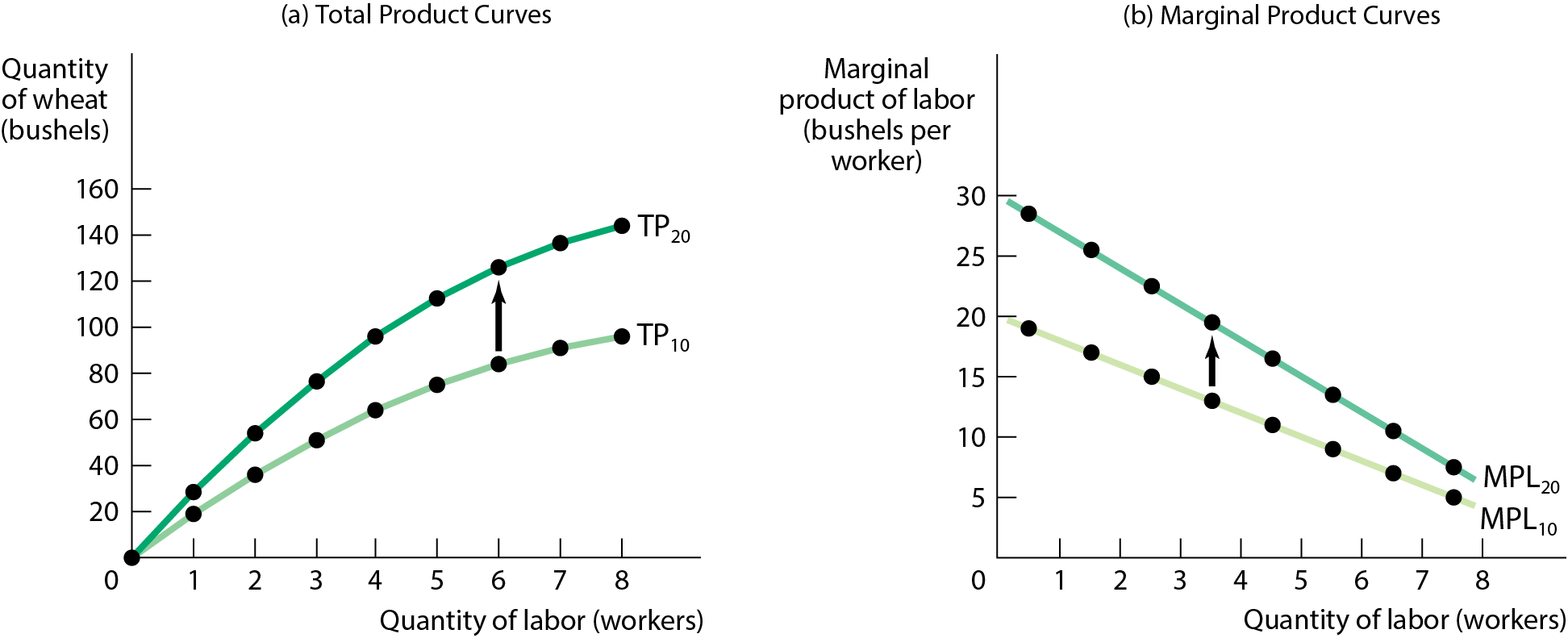
Total product, marginal product, and fixed input
With more land (fixed input), each worker can produce more. This shifts the total product curve up
So the MPL of each worker is higher when the farm is larger, and the MPL curve shifts up too
Pitfalls: What is a unit
The MPL is defined as the increase in the quantity of output when you increase the quantity of that input by one unit
What do we mean by a unit of labor? Is it an additional hour of labor, an additional week, or a person-year?
The answer is that it doesn't matter, as long as you are consistent
From the production function to cost curves
A fixed cost is a cost that does not depend on the quantity of output produced. It is the cost of the fixed input
A variable cost is a cost that depends on the quantity of output produced. It is the cost of the variable input
Total cost curve
The total cost of producing a given quantity of output is the sum of the fixed cost and the variable cost of producing that quantity of output
TC = FC + VC
The total cost curve shows how the total cost depends on the quantity of output
The total cost curve becomes steeper as more output is produced, a result of diminishing returns
With diminishing returns, additional units of output require more and more labor; therefore, the cost increases
Total cost curve graphed
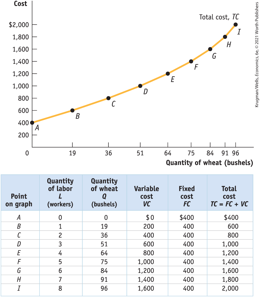
The curve gets steeper as output increases due to diminishing returns to labor
Marginal cost
The marginal cost if the change in total cost generated by one additional unit of output
MC = ΔTC/ΔQ
Where Δ = change, TC = total cost, and Q = quantity of output
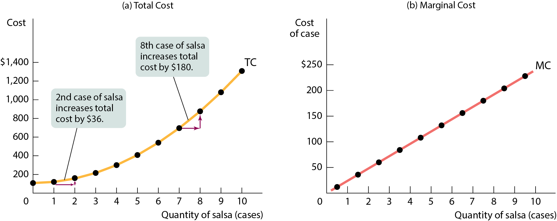
Why is the marginal cost curve upward sloping
Because there are diminishing returns to input in this example. As output increases, the marginal product of the variable input declines
This implies that more and more of the variable input must be used to produce each additional unit of output as the amount of output already produced rises
And since each unit of the variable input must be paid for, the cost per additional unit of output also rises
Average cost
Average total cost (often referred to simply as average costs) = total cost per unit of output produced
ATC = TC/Q
Average fixed cost = fixed cost per unit of output produced
AFC = FC/Q
Average variable cost = variable cost per unit of output produced
AVC = VC/Q
Average total cost curve
Increasing output has two opposing effects on the average total cost
The spreading effect: the larger the output, the more output over which the fixed cost is spread, leading to a lower average fixed cost
Diminishing returns effect: the larger the output, the more variable input required to produce additional units, which leads to a higher average variable cost
Putting the four cost curves together
Note that
Marginal cost slopes upward because of diminishing returns
Average variable cost also slopes upward, but is flatter than the marginal cost curve
Average fixed cost slopes downward because of the spreading effect
The marginal cost curve intersects the average total cost curve from below, crossing it at its lowest point
Minimum average total cost
The minimum cost output is the quantity of output at which average total cost is lowest – the bottom of the U-shaped average total cost curve
Three general principles are always true about a firm's marginal cost and average total cost curves
At the minimum cost output, the average total cost is equal to the marginal cost
At output less than the minimum-cost output, the marginal cost is less than the average total cost, and the average total cost is falling
At output greater than the minimum cost output, the marginal cost is greater than the average total cost, and the average total cost is rising
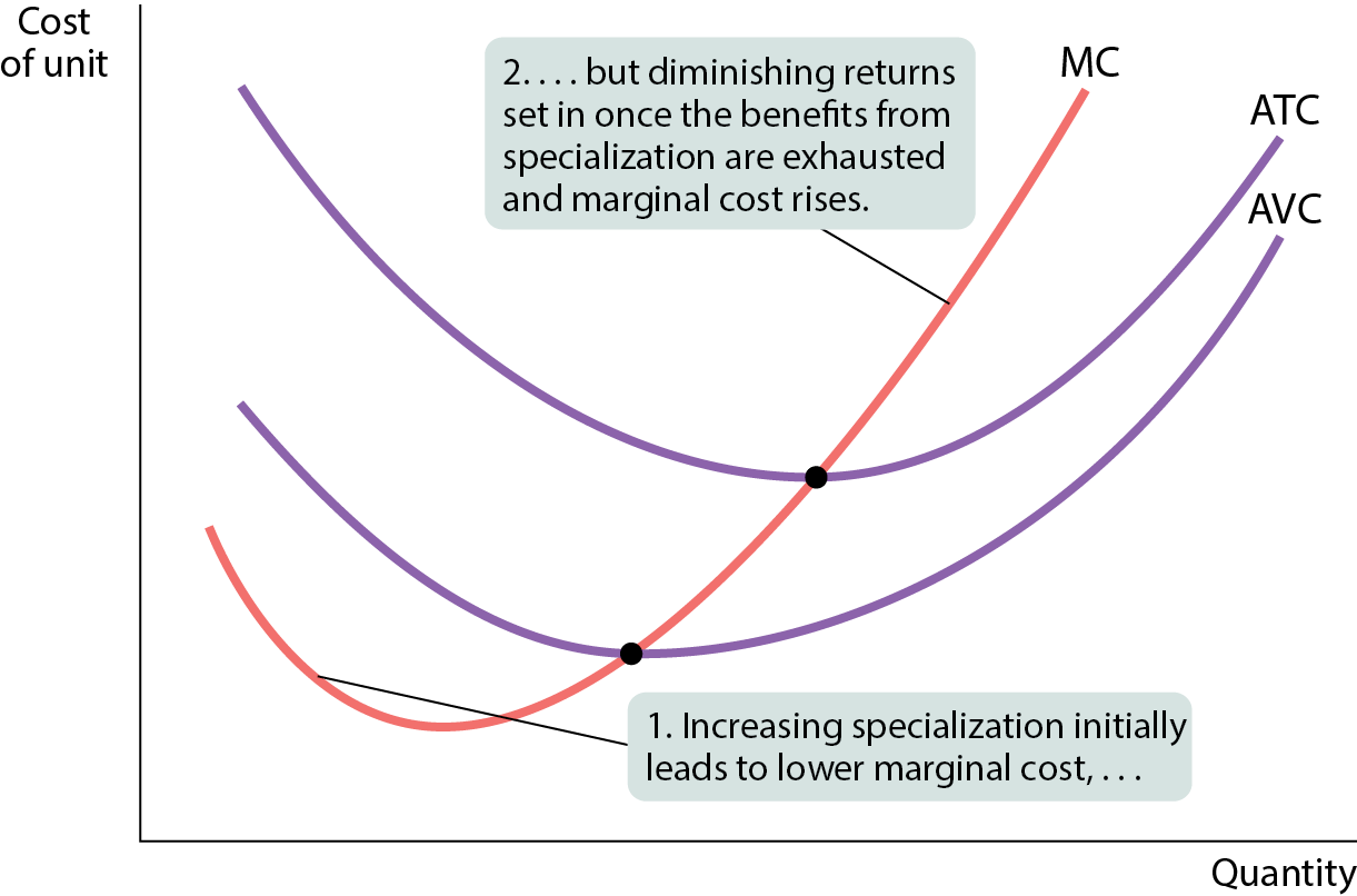
Does the marginal cost curve always slope upward?
Marginal cost curves often slope downward as the output goes from zero up to some low level, and they slope upward at higher levels of production
The initial downward slope occurs when employing more workers allows them to specialize in various tasks
This specialization leads to increasing returns to the hiring of additional workers and results in the marginal cost curve sloping downward
Once enough workers exhaust the benefits of specialization, diminishing returns to labor set in, and the marginal cost curve slopes upward
Typical marginal cost curves have the “swoosh” shape
Short-run versus long-run costs
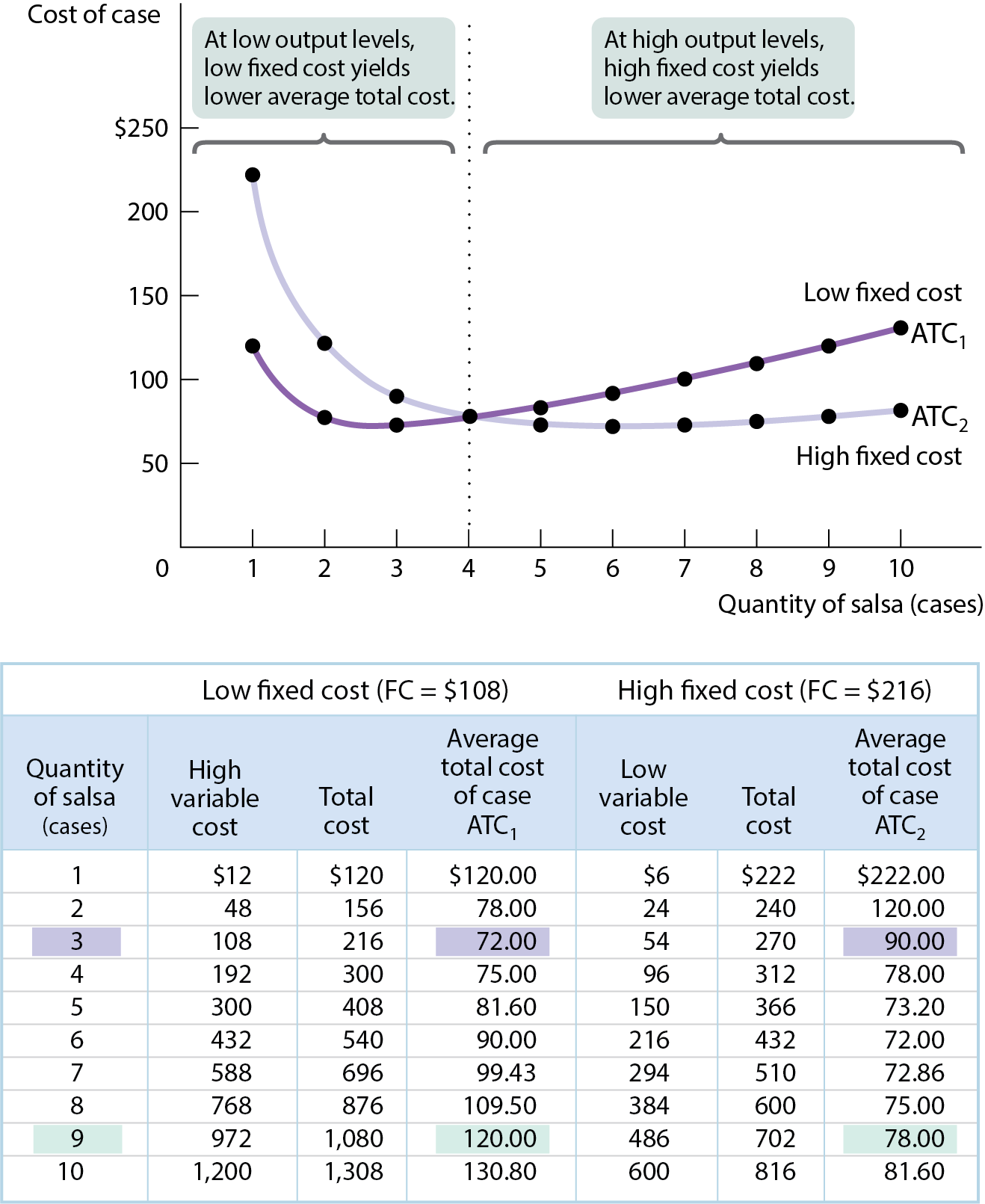
All inputs are variable in the long run. This means that in the long run, fixed costs (like factory size) may also vary
The firm will choose its fixed cost in the long run based on the level of output it expects to product
Choosing the level of fixed cost
There is a trade-off between higher fixed costs and lower variable costs for any given output level, and vice versa
The long-run average total cost curve
The long-run average total cost curve shows the relationship between output and average total cost when fixed cost has been chosen to minimize average total cost for each level of output
We assume the firm has chosen the cheapest plant size for each output level
Short-run and long-run average total cost curves
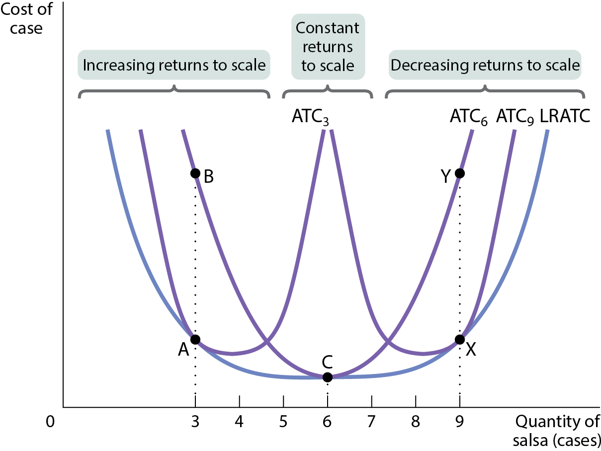
Short-run and long-run average total cost curves differ because a firm can choose its fixed cost in the long run.
If the firm chooses the fixed cost that minimizes short-run ATC at an output of 6, and produces 6, it’s at point C.
If it produces only 3, it’ll move to point B.
If the firm expects to produce 3 cases for a long time, it’ll reduce its fixed cost and move to point A. If it produces 9 (point Y) and expects to continue at this level for a long time, it’ll increase its fixed cost and move to point X.
Return to scale
There are increasing returns to scale (economies of scale) when the long-run average total cost declines as output increases
There are decreasing returns to scale (diseconomies of scale) when the long-run average total cost increases as output increases
There are constant returns to scale when long run average total cost is constant as output increases
Chapter 15: Perfect competition and the supply curve
What will we learn in this chapter?
What is perfect competition and why do economicsts consider it an important benchmark
What factors make a firm or an industry perfectly competitive?
How does a perfectly competitive industry determine the profit-maximizing output level?
What determines if a firm is profitable or unprofitable?
Why does it make sense for a firm to behave differently in the short run versus the long run?
How does the short-run industry supply curve differ from the long-run industry supply curve?
Defining perfect competition
All market participants, both consumers and producers, are price-takers
There are many producers, each with a small market share
Market share: the fraction of the total industry output accounted for by that producers output
This means both sellers and buyers are price-takers; their actions have no effect on price
Each participant is a drop in the bucket
Consumers regard the products of all producers as equivalent
The product is standardized across sellers
Standardized product (aka commodity): consumers regard different sellers’ products as the same
Free entry and exit
Most eprfectly competitive industries are also characterized by free entry and exit
New producers can easily enter into an industry, and existing producers can easily leave that industry
Production and profits
Each firms total revenue is equal to price x quantity sold
TR = P x Q
And profit = total revenue - total cost
Profit = TR - TC
What market price = $72, profit is highest at Q = 50
Margianl profit analysis and the profit maximizing output
Recall the profit maximizing principle of marginal analysis: the optimal amount of activity is the level at which marginal benefit equals marginal cost
Marginal revenue = change in total revenue egeneraterd by an additional unit of output
Always just cost
MR = ΔTR/ΔQ
Since the firm is a price-taker, MR equals the price: the firm can sell as much as it likes at the current market price. Its marginal revenue curve is a horizontal line at the market price
Since the firm is a price-taker, the firm faces a horizontal, perfecty elastic demand curve that is equivalent ti its marginal revenue curve
Optimal output rul: profit is maximized by pridcuing the quantity of output at which the marginal revenue of the last unit produced is equal to its marginal cost
Why is profit maximize where MR = MC
Each time the firm producers another unity, there are extra costs and extra revenues
If producing another unit adds more revenue than it costs, profit will increase
If MR > MC, producing more will add to profit
If MR < MC, producing less will add to profit
Since MR = P for competitive firms, the profit-maximizing rule is to choose the quantity of output where P = MC
Pitfalls
What if marginal revenue and marginal cost aren’t exactly equal
What do you do if there is an output level at which ,argianl revenue equals marginal cost
In that case, you produce the largest quantity for which margincal revenue exceeds marginal cost
When is production profitable
Recall that we are using economic profit – the profit that includes the implicit cost (the forgone benefits of the firm’s resources) and the explicit cost (cash outlays)
If TR > TC, the firm is profitable
If TR = TC, the firm brekas even
If TR < TC, the firm incurs a loss
We can express this idea in terms of avg. revenue and cost per unit of output
If the firm produces a quantity at which P > ATC, the firm is profitable
If the firm produces a quantity at wich P = ATC, the firm breaks even
If the firm producers a quantity at which P < ATC, the firm incurs a loss
Cost and production in the short run
Profitability and the market price
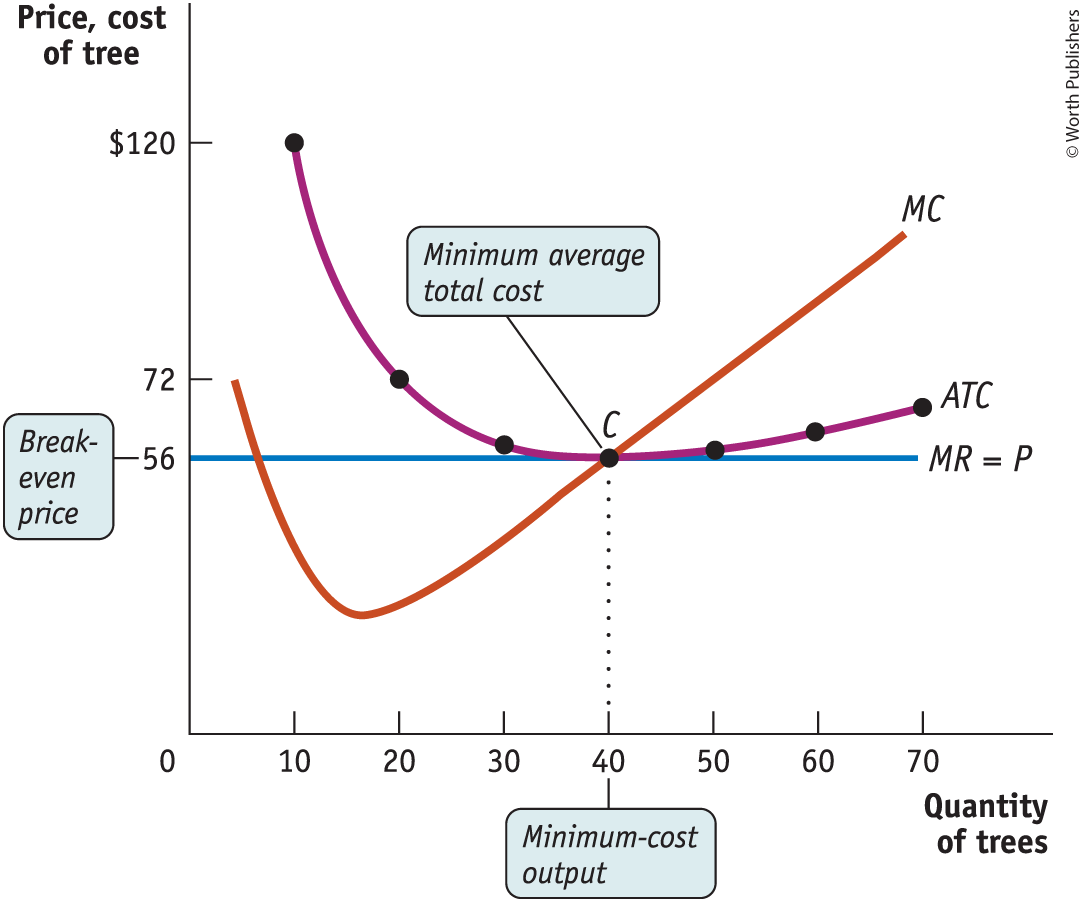
The firm is profitable because P > min ATC
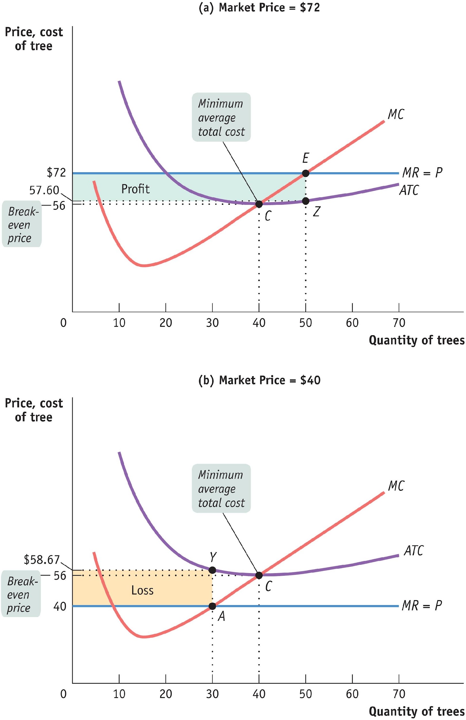
The farm’s per unit profit
%72 - $57 = $14.40
Total profit 50 x $14.40 = $720
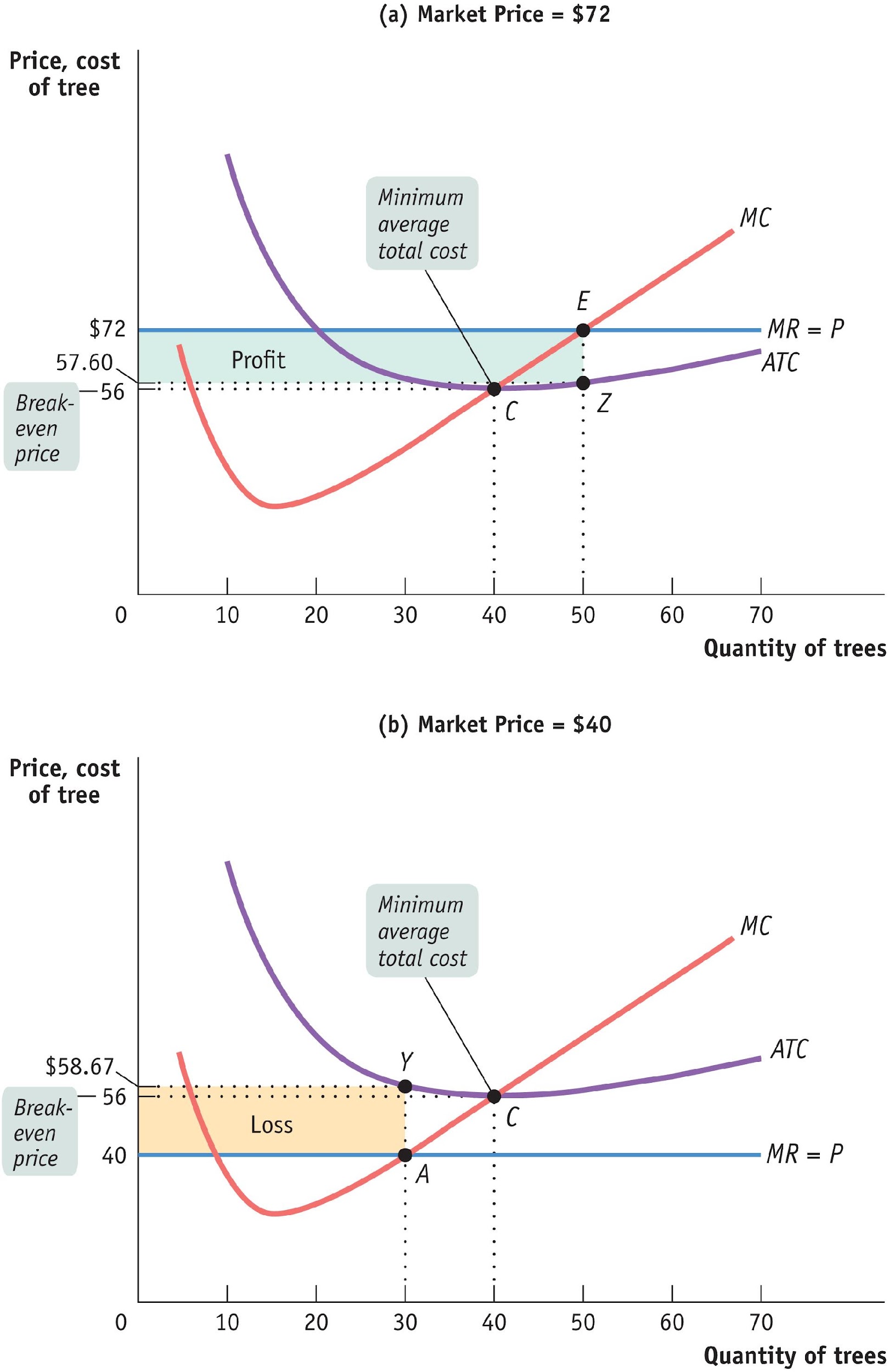
The farms per unit loss: $58.67 - $40 = $18.67
Total loss: $30 x $18.67 = $560
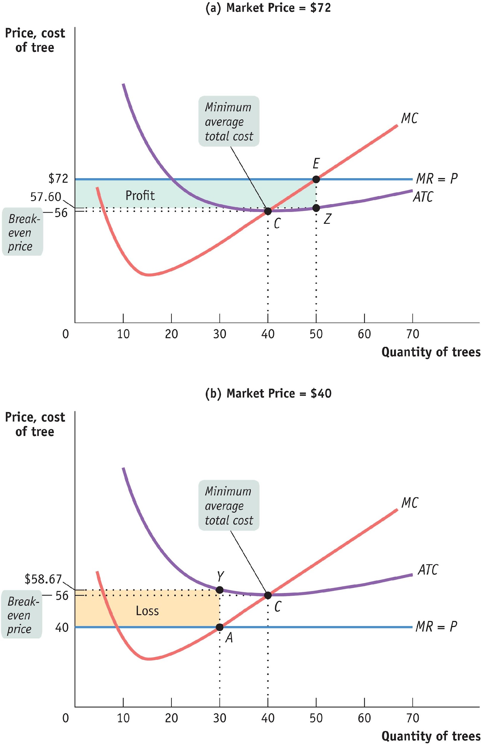
Calculating total cost and profit
Profit = TR - TC (TR/Q -TC/Q) x Q
Profit = (P - ATC) x Q
The break even price of a price taking furm is the market price at which it earns zero profit
The short- run production decision
Looses don’t mean immediate shutdown
Fixed costs must be apid regardless of whether the firm producers in the short run
Snce it cannot be changed, fixed costs is irreverent to the decision about whether to shut down in the short run. Other costs – variable costs – do matter
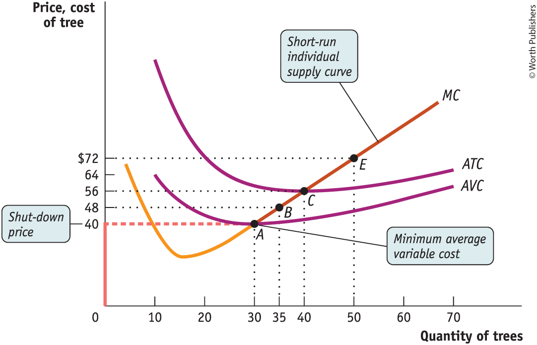
When the market price is below minimum average variable cost, a firm should cease production immediately. The minimum avg. variabe cost is equal to the shut-down price
When price is greater than minimum avg. variable cost, however, the firm should produce in the short run
The short-run individual supply curve
A firm will produce at every precise avboeb minimum ATC where prie intersects the MC curve…. But will stop producing in the short run if the market price falls below the shut-down roice,, so thew MC curve (above shut-down price) is the firm’s supply curve
Changing fixed cost
Buying or selling equipment allows a firm to change iys fixed cost
A firm w ill choose the level of fixed cost that minimizes the average totoal cost for its desired output quantity – an that may mean closing down altogether
The short run industry supply curve
The industry supply curve shows the relationship between the price of a good and the total output fo the industry as a whole
The fort run industry supply curve shows how the quantity supplied by an industry depends on the market price given a fixed number of producers
There is a short run market equilibrium wen the quantity supplied equals the quantity demanded, taking the number of producers as given
The short run market equilibrium
The short run market equilibrium the quantity supplied equals the quantity demanded, taking the number of producers as given
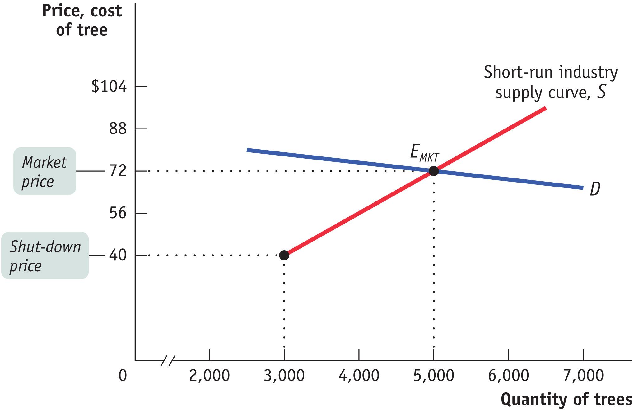
The long run market equilibrium
New firms enter as long as there si economic profit ( P> min ATC)
A market is in the long run equilibrium when the quantity supplied equals the quantity demanded, given that sufficient time had elapsed for entry into and exit from the industry to occur
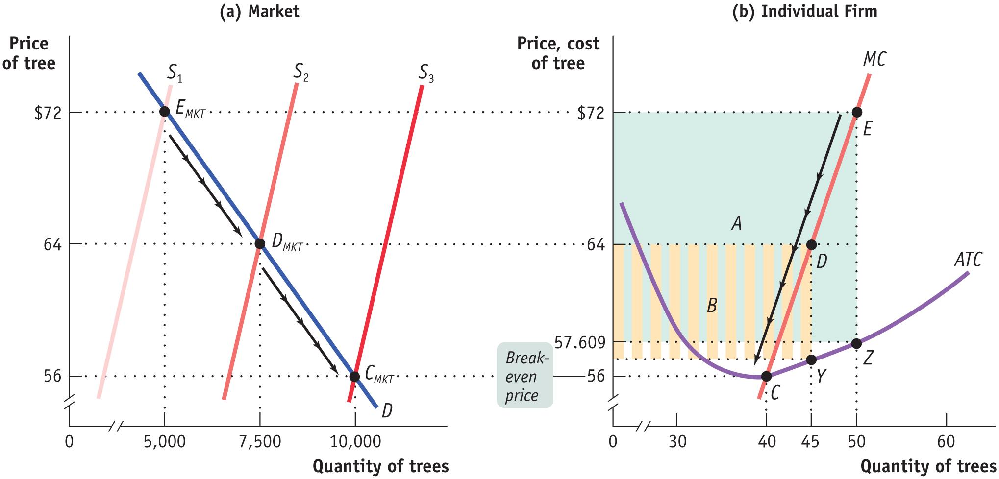
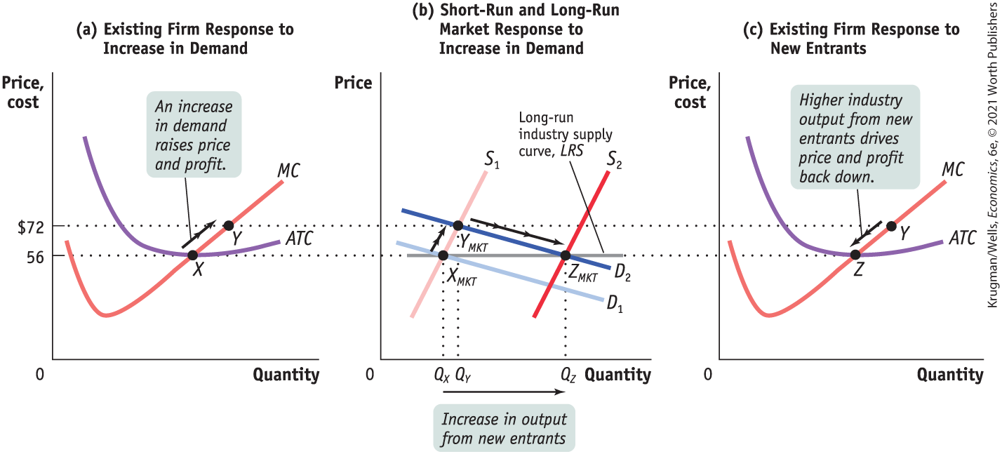
The effect of an increase in demand in the short run and the long run
The LRS shows how the quantity supplied responds to the price (once producers have had the time to enter or exit the industry
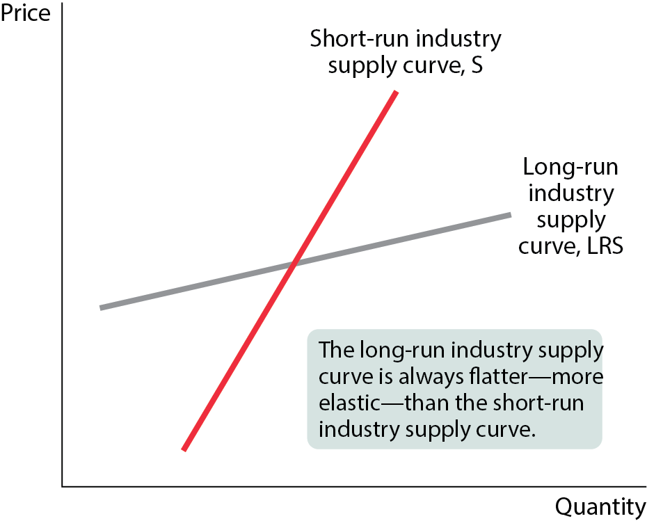
Comparing the short run and long run industry supply curves
The long-run supply curve is flatter than the short-run supply curve
A higher price attracts new entrants in the long run, raising industry output and lower cost
A fall in price induces existing producers to exiting in the long run, reducing industry output and rasing price
The long run industry supply curve
The long-run supply curve is perfectly elastic if costs are constant across the industry—if each firm, be it an incumbent or a new entrant, faces the same cost structure. Example: agriculture in which there is a perfectly elastic supply of inputs.
The long-run industry supply curve slopes upward when producers use an input that is in limited supply. As the industry expands, the price of that input goes up, and later entrants have a higher cost structure than early entrants. Example: beachfront resort hotels, which compete for a limited quantity of prime property. Such industries are said to have increasing costs.
Industry supply curve slopes downward when an industry faces increasing returns to scale, in which average costs fall as output rises.
Whether the long-run industry supply curve is horizontal or upward sloping or even downward sloping, the long-run price elasticity of supply is higher than the short-run price elasticity whenever there is free entry and exit.
Pitfalls
Economic profit, again
Why would a firm want to enter an industry if the market price is only slightly greater than the break even price?
We are usinhg economic profits as our measure, so if the market price is above the break even level (no matter hwo slightly), the firm can earn more in this idnsurty than it could elsewhere
Chapter 16: Monopoly
What will we learn in this chapter?
What is the significance of monopoly, a type of industry in which only one producer, a monopolist, operates?
How does being a monopolist affect a firm’s price and output decisions?
Why does the presence of monopoly typically reduce social welfare?
What tools do policy makers use to address the problem of monopoly?
What is price discrimination, and why is it so prevalent in certain industries?
How do digital giants like Amazon, Google, and Meta fit into our model of monopoly, and what special challenges do they represent?
Types of market structure
In order to develop models abd make predictions about how producers will behave, eonomists have developed four principle models of market structured
Perfect competition
Monopoly
Oligopoly
Monopolistic competition
This system of market structures is based ont wo dimensions
The number of firms in the market (one, few, or many)
Whether the goods offered are identical or differentiated
The meaning of monopoly
Monopolist: a firm that is the only rpduers of a good with no close substitutes
Monopoly: a industry controlled by a monopolist
Market power: the ability of a firm to raise prices
What a monopolist does
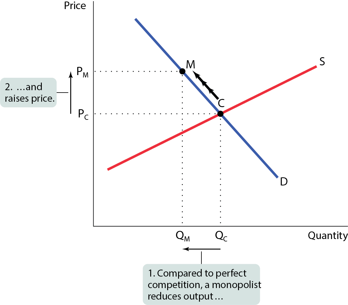
A monopolist reduces the quantity supplied to Qm and moves up the demand curve from C to M, raising the price to Pm
Why do monopolies exist
For a monopoly to persist, something must keep othgers from going into the same business: a barrier to entry
There are 5 principal types of barries to entry
Control of scarce resource or input
Increasing returns to scale
Technological superiority
Network externaltities
Governemtn-made barriers
Barrier #1: control of a scarce resource or input
A monopolist that controls a crucial resource or input can prevent other firms from entering its market
Barrier #2: increasing returns ro scale
Increasing returns to scale (economies of scale): whena verage total costs falls as output increases, firms tend to grow larger
The source of increasing returns to scale is large fixed coss
In surch an industry, larger companies are more profitable and drive out smaller ones
Increasingr returns to scae can give rise to and sustain monopoly
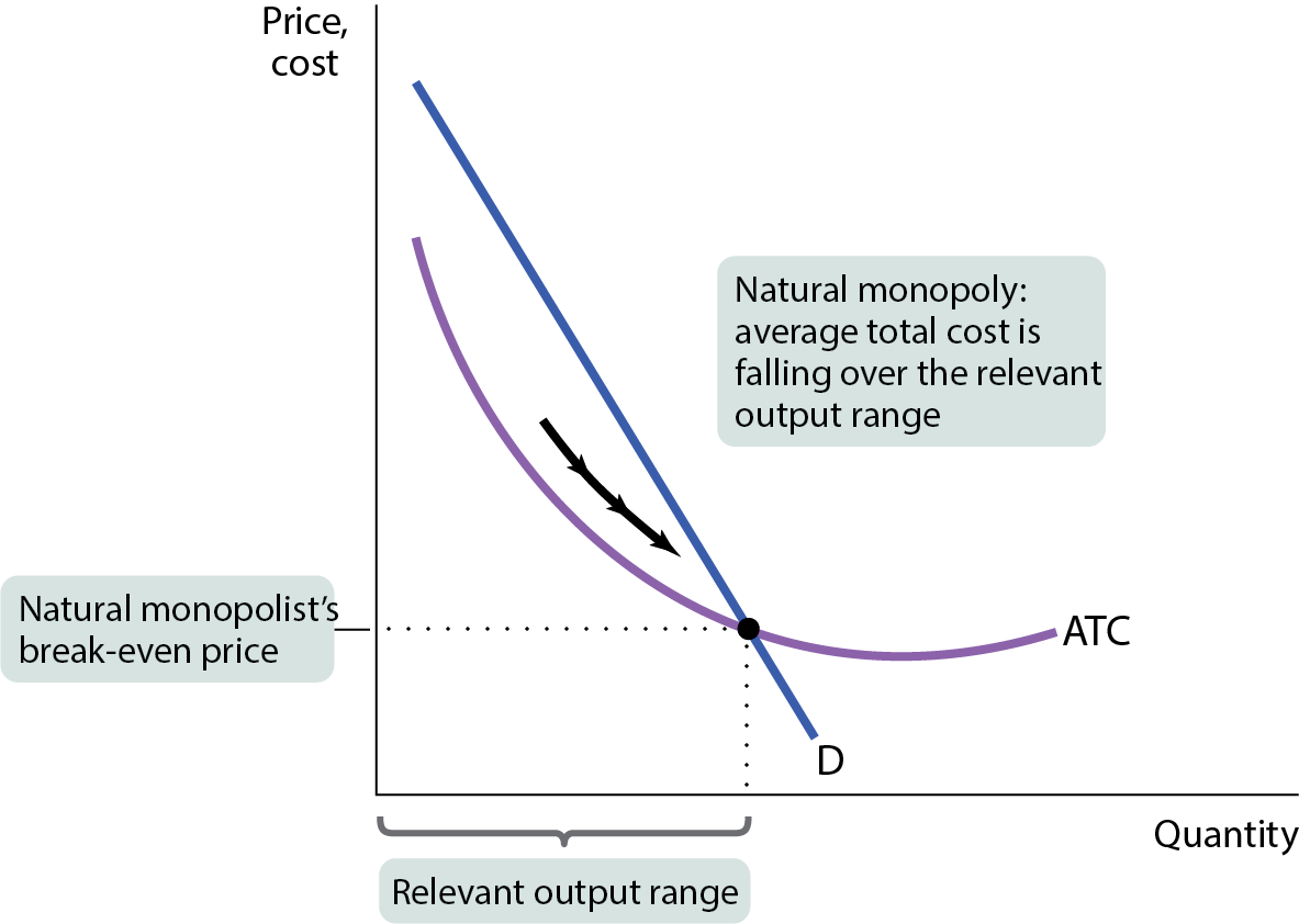
A monopoly created and sustained by increasingr returns to scale is called a natural monopoly
The most visible natural monopolies are utilities – water, natural gas, power generation, and fiber optic cable
Barrier #2 in a graph
A given quantity of output is proiduced more cheaply by one larger firm than by two or more smaller firms
Barrier #3: technological superiority
A firm that maintains a consistent technologica advantage over potential competitors can establish itself as a monopolist
Ex. Intel was technologically superior over other firms from the 1970s to the 1990s
Technological superiority is typically nto a barrier to entry over the longer term
Barrier #4: network externality
Network externality: the value of a good or service to an individual increases as more individuals use the same good or service
The firm with the largest network of customers may become a monopoist
Ex. ebay, meta, amazon, netflix, google, venmo, and tiktok
Barrier #5: government-created barrier
A patent gives an inventor a temporary monopoly in the sue or sale of an invention
A copyright gives the creator of a literary or artistic work sole rights to proffit from that work
The justification for patents and copyrights is a matter of incentives: The law allows a monopoly to exit temporarily by granting property rights that encourage invention and creation
Global comparison: drug prices
Different drug prices in different countries reflect willingness to pay; they also reflect that governments in toher ocutnries regulate drug prices more actively thsn the U.S. government does
How a monopolist maximizes profit
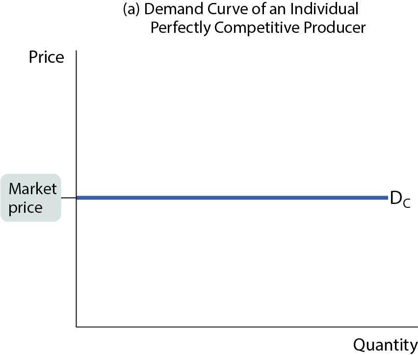
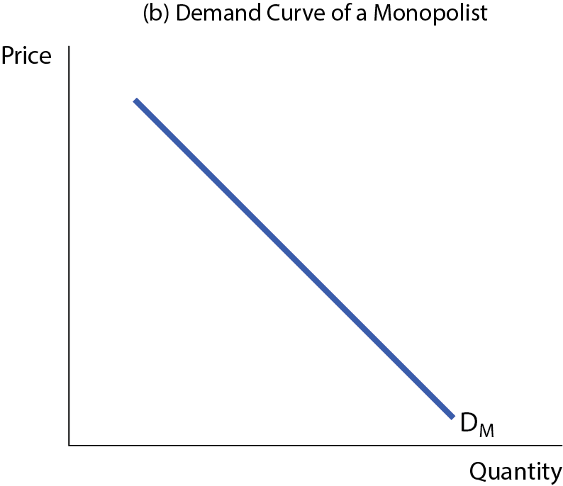
Competitive firms can’t choose price
Monopolist can
Profit-maximizing rule
All firms allow the same rule: profit is maximized at the Q where Mr = MC
So what does MR look like
MR = ∆TR / ∆Q
Marginal revenue and the demand curve
MR is below the demand curve
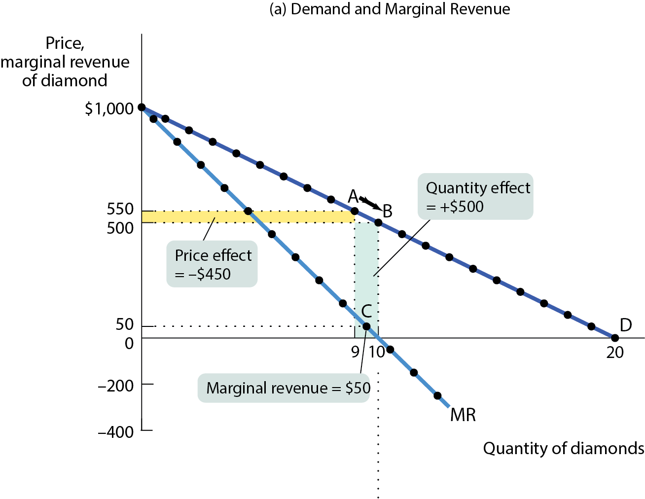
An increase in production by a monopolist has two opposinge effects on revenue
A quantity effect: one more unit is sold, increasing total revenue by the price at which the unit is sold
A price effect: to sell the last unit, the monopolist must chut the market price on all units sold; this decreases total revenue
A monopolist’s marginal revenue curve is always below the demand curve because of the price effect: To sell an additional unit, the monopolist must cut the market price on all units sold
A monopolists demand, total revenue, and marginal revenue curves
Profit maximization for a monopoly
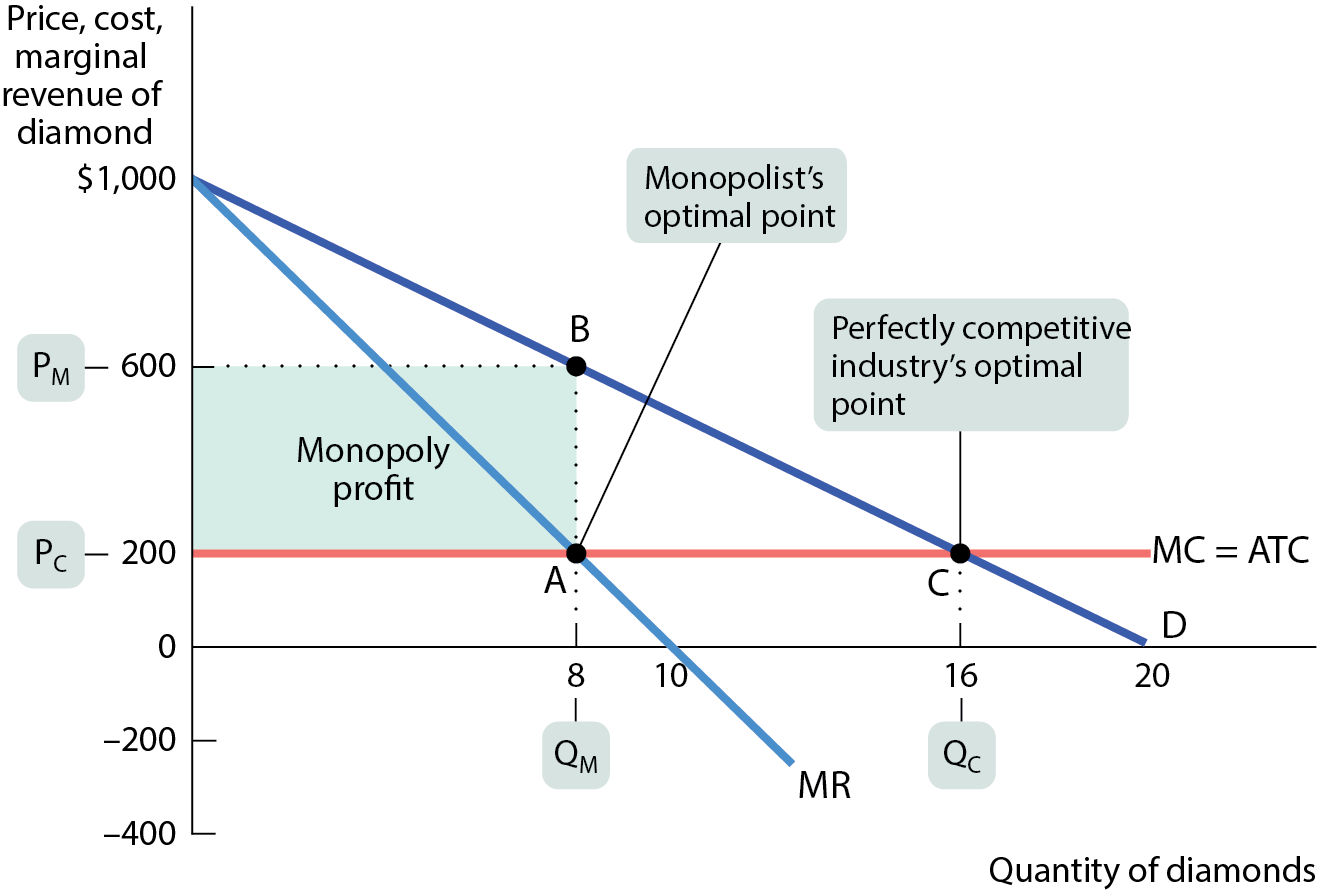
Profit maximization consists of two steps
Choosing a quanittuy
Rule: choose Q where MR = MC
Choosing a price
Choose the highest price you can get away with, which is the high price consumer will pay for that quantity
Rule: one you’ve picked your quantity, follow the graph to the demand curve, whci shows how much consumers will pay
The monopolist’s profit-maximizing output and price
Note: here the MC curve is simopified to be constant. We will relax this simplification later
Pitfalls findinaing the monopoly price
In order to find the profit-maximizing quantity of output for a monopolist, you look for the pint where MR curve crosses the MC curve
But this isn’t the price the monoplost will choose. The firm will want to charge as much as it can
Why stop at MR if it can charge up tot what the demand curve says people will pay
Graphing the monopolist's profit
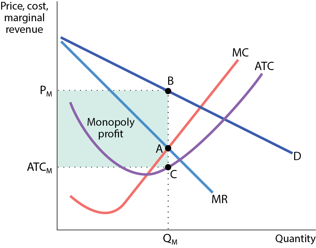
As long as the monopoly hads strong barriers to entry, profit will stay
Pitfalls: is there a monopoly supply curve
You might eb tempted to ask about the supply curve of a monopolist. But this is a meaningless questions
Monopolists doen’t have supply curves – since they control prices there is no set relationships between price and quantity supplied
Monopoly and public policy
A monopolist, by reducing otuput and raising prices, ebenfits at the expense of consumers
Monopoly is a source of inefficiency, the losses to consumers from monopoly behavior are larger than the gains to the monopolist
Monopoly leads to net losses to society’s welfare
Governments ofnten try to either prevent or to limit monopolies
Monopoly causes inefficiceny
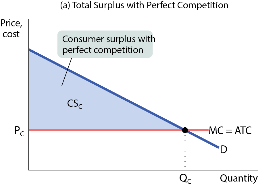
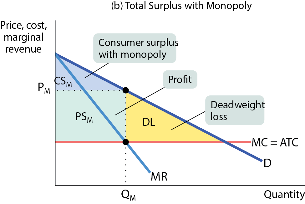
Panel (a), perfect competition: since price equals the producer’s ATC, there’s no profit and no producers surplus. Total surplus, equal to consumers surplus, soi the entire shaded area
Panel (b), monopoly: the monopolist decreases output to Qm and changes Pm. the blue area shows consumer surplus, the green area shows profit; and the yellow area is a deadweigth loss. As a result, total surplus falls
Policy remedies to monopoly
If its a natural monopoly or a network externality industry, bigger is better for a consumer. These monopolies provide value from consumers
If neither of those conditions apply, the ebay policy is to prevent monolply from arising ro to bresak it up if it already exists
The government policies used to prevent or limit onoploies are know as antitrust policies
Dealing with natural monpoly
Natural monopolies are a different story: a larger producrs has lower average total cost than small producers and shouldn’t be broke up
Yet, even a natural monopolist causes inefficiencies. Two policy options
Public ownership the governembt establishes a public agnecy to provide the good and protect consumers’ interest. This solution often works badly because publicly owned company are often poorly run
Regulation: a price ceiling imposed on a monopolist does not create shortages if it is not set too low
Unregulated and regulated natural monopoly
If the monopoly’s price is regulated at Pr, consumer surplus rises (and profits fall)
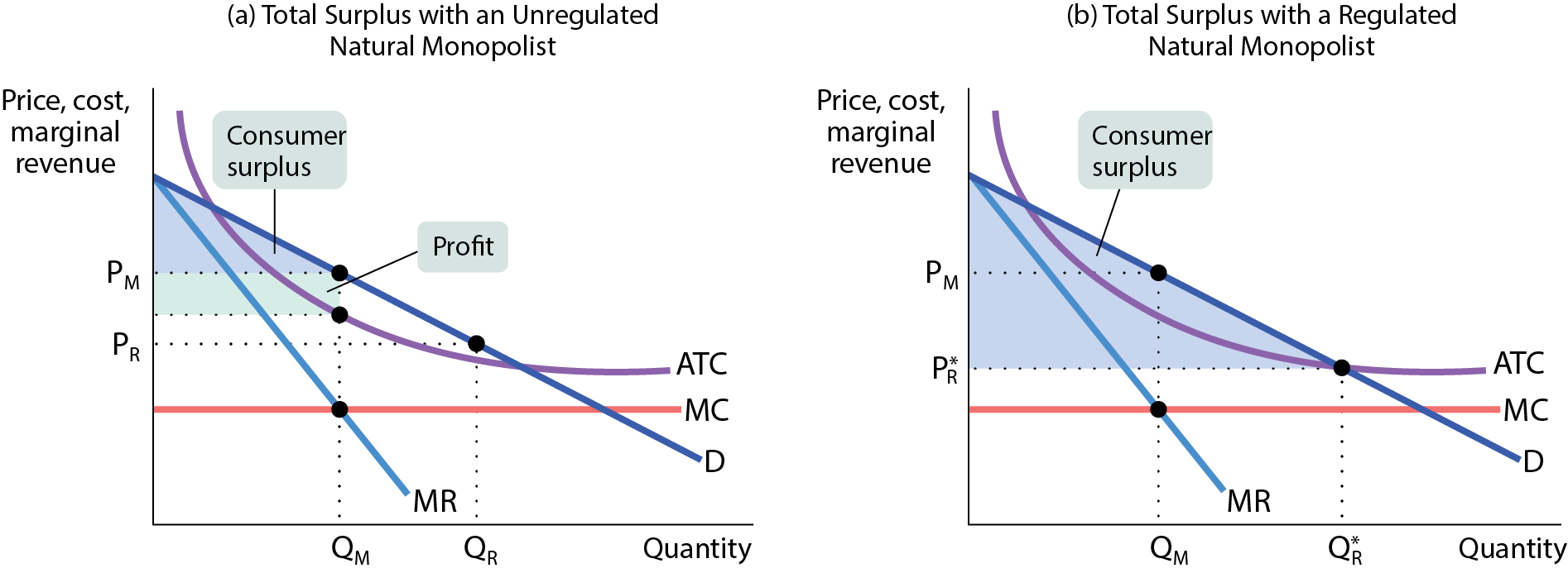
Price discrimination
So far we’ve been assuming our firm is a single-price monopolist: it offers its product to all consumers at the same price
Some firms practice price discrimination: they charge different prices to different consumers for the same good
Price discrimination and profit maximization
Recall the profit-maximizing rule for firms with monopoly power
Produce the Q at which MR = MC
Based on that Q, charge as much as the market will bear (found by the position of the demand curve)
But what if you sell more than one market, each with its own demand curve
Ex. senior citizens and young people, business travelers and leisure travelers
The logic of price discrimination
If the airline could charge two types of customers two different orices, it wouldncapture of all the consumer surplus as profit
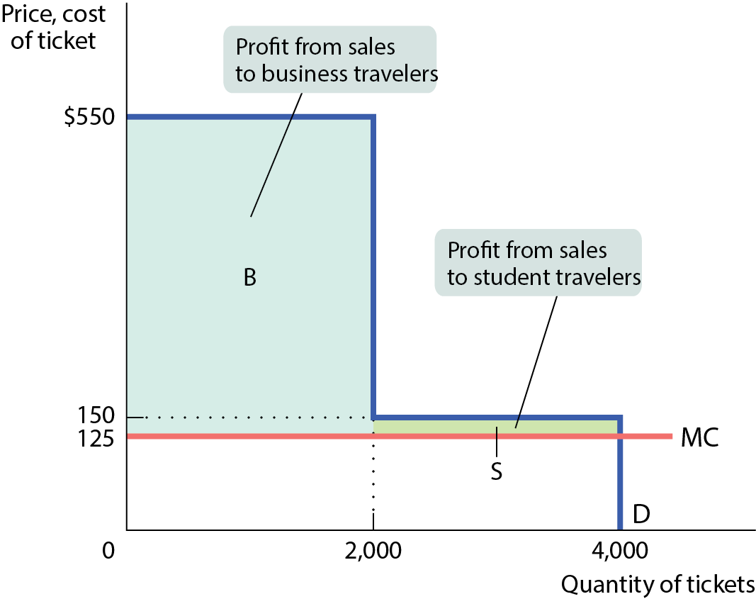
Price discrimination and elasticity
Firms would distinguish between groups of customers on the basis of their sensitivity to the price – their price elasticity of demand
Example: Business travelers have lower price elasticity of demand than nonbusiness travelers. Airlines impose rules that indirectly charge business and nonbusiness travelers different fares: fares are higher if you don’t stay over a Saturday night.
Price discrimination increases sales and profits
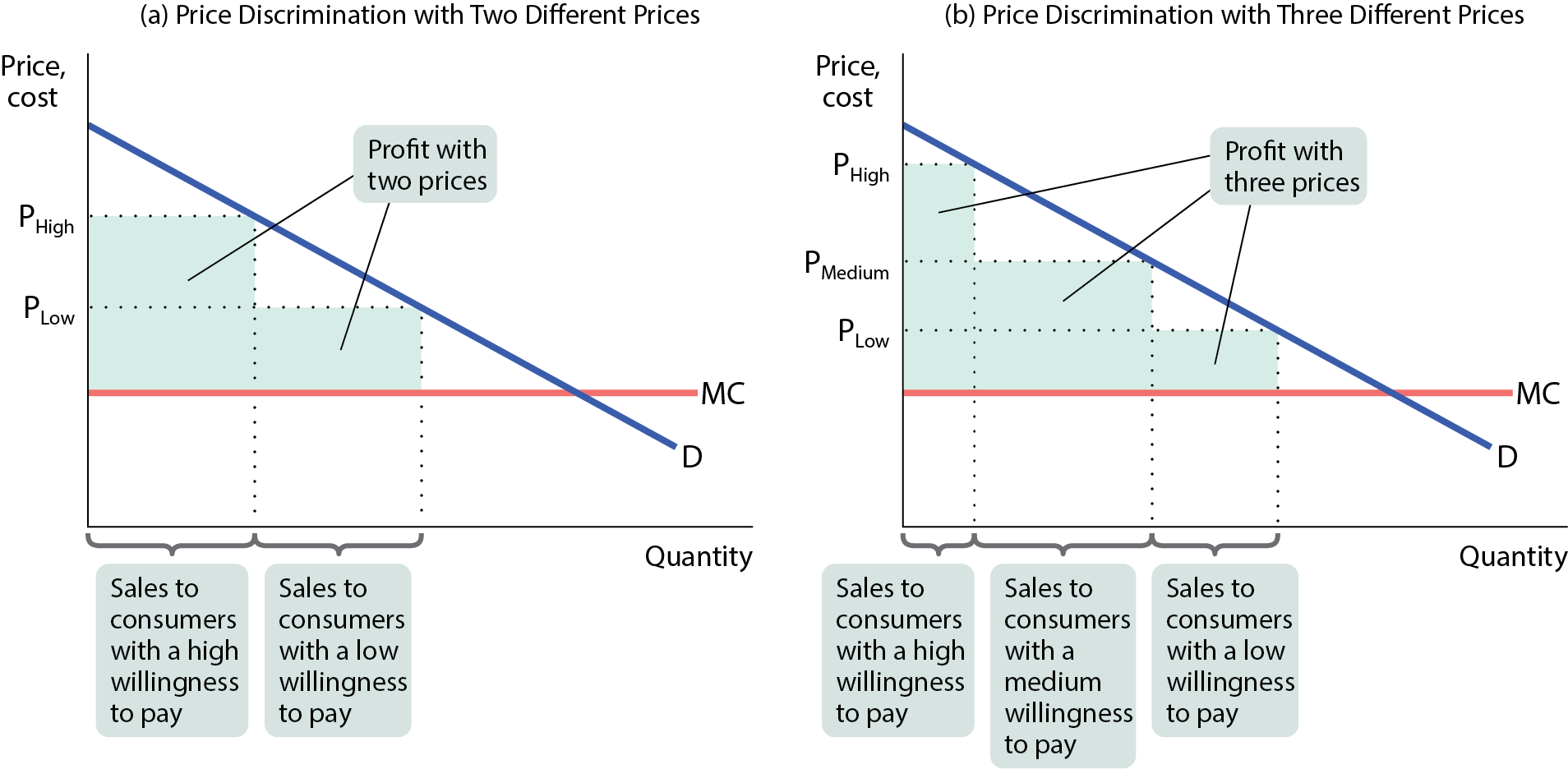
Perfect price discrimination
When perfect price discrimination can be employed, a firmw ill charge each customer a diffeent price, the maxmimum price each is willing to pay
Under perfect price discrimination, the firm captures all consumer surplus as profit
Handling at the flea market: perfect price discrimination
Graphing perfect price discrimination
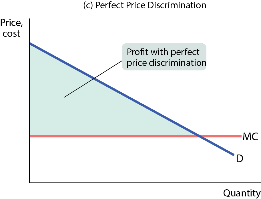
There is no deadweigth lsos because all mutually ebenficial transactions are exploited
There is zero consumer usrplus becaise th eentire surplus si acptures bu the monopolist in the form of profit
Common techniques for price discrimination
Advance purchase restrictions
Prices are lower for those who purchase well in advance
Volume discounst
The price is lower if you buy a larger quantity
Two-part tariffs
A customer pays a flat fee upfront and then a per-unti fee on each item purchased
Sales and otuelt stores
Holding regular sales such as black friday saes, labor day sales, and so on; building an otulet store at a distance from the center of the city
Bigital personalized pricing
Inline retailers gather personal ifromation on shoppers and adjust prices accordingly
A new generation of market power
The rise of the digital economy and the network externalisites provide new ways of gaining market power and becoming a monopolist: facebook, microsoft, apply, google, ebay, uber, paypal
Bigger is better”: the biggest firm in the industry gets bigger, while smaller firms shrink.
The dominant firm creates a deadweight loss and another inefficiency: stifling innovation.
A federal court found Microsoft guilty of using its market dominance against rivals. The EU’s antitrust authorities accused Google of stifling innovation by blocking rivals across platforms.
Monopsony
A monopsony exits when there is only one buyer of a good
The classic example is a single employer in a small twon that is hiring workers
Like a monopolist, a monopsonist distorts the competitive market equilibrium and create a deadweigth loss
Apple is currently the subject of several snti-trust cases, witg may claiming that the Apple App store is an example fo monospony behavior arinsing froma network externality
Chapter 17: Oligopoly
What will we learn in this chapter?
What is oligopoly, abd why does it occur
Why do oligopolists benefit from collusion,a nd how are consumers hurt by it
How do the insights gained from game theory helpus to understand the strategic behavior of oligopolists
Why is antitrust policy—policy which is aimed at preventing collusion among oligopolists—a critical function of government?
The prevelance of oligopoly
An oligopoly is a market that is dominated by a small number of firms.
A firm in such an industry is known as an oligopolist.
Economists refer to a situation in which firms compete but also possess market power—which enables them to affect market prices—as imperfect competition.
Two forms of imperfect competition: oligopoly and monopolistic competition.
Why are oligopolies so prevalent?
Oligopoly is the result of the same factors that produce monopoly, but in weaker form. The most important one is the existence of increasing returns to scale.
When these effects are very strong, they lead to monopoly; when they are moderately strong, they lead to oligopoly.
To get a better picture of market structure, economists often use the Herfindahl–Hirschman Index, or HHI.
The HHI for an industry is the sum of the squares of each firm’s share of market sales.
For example, if there are three firms with 60%, 25%, and 15% market share each:
HHI = 602 + 252 + 152 = 4,450
HHI of less than 1,000 indicates a strongly competitive market.
HHI of 1,000 to 1,800 indicates a somewhat competitive market.
HHI above 1,800 indicates an oligopoly.
If HHI is above 1,000, a merger that results in a significant increase in the HHI will receive special scrutiny and is likely to be disallowed.
Understanding oligopoly
Oligopolists operate in a state of interdependence: the decisions of one firm affect the profits of its rivals.
An oligopoly consisting of only two firms is a duopoly. Each firm is known as a duopolist.
Sellers engage in collusion when they cooperate to raise their joint profits. A cartel is an agreement among several producers to obey output restrictions in order to increase their joint profits.
The world’s most famous cartel is the Organization of Petroleum Exporting Countries (OPEC).
Collusion and competition
Will oligopolists engage in collusion or in noncooperative behavior?
Noncooperative behavior: each firm acts in its own self-interest, and firms ignore the effects of their actions on each others’ profits.
Collusion between firms is illegal, but sometimes firms ignore the rules and collude.
By acting as if they were a single monopolist, oligopolists form a cartel.
Each firm has an incentive to cheat and produce more. There are two principal outcomes: successful collusion or behaving noncooperatively by cheating.
Games oligopolist play
Each oligopolist realizes that it is interdependent: its profit depends on what its competitor does, and its competitor’s profit depends on what it does.
The firms are playing a game in which the profit of each player depends not only on its own actions but on those of the other players.
To understand how oligopolists behave, economists and mathematicians developed game theory.
Game theory: the study of behavior in situations of interdependence; a way of predicting outcomes in strategic situations like oligopolies.
The prisoners’ dilemma
The reward received by a player in a game, such as the profit earned by an oligopolist, is that player’s payoff.
A payoff matrix shows how the payoff to each of the participants in a two-player game depends on the actions of both.
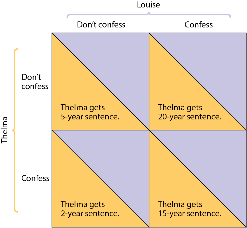
The prisoners’ dilemma: Thelma and Louise are caught by the police. The police put them in separate cells and say, “If neither of you confesses, we’ll send you to jail for 5 years. If you confess and implicate your partner, and she doesn’t do the same, we’ll reduce your sentence from 5 years to 2. But if your partner confesses and you don’t, you’ll get the maximum 20 years. If both of you confess, we’ll give you both 15 years. And if you both remain silent, we’ll give you 5 years each.”
Both prisoners will confess.
To confess is a dominant strategy: the player’s best action regardless of the action taken by the other player.
The prisoners’ dilemma is a situation when each player has an incentive to cheat and both players end up being worse off.
A Nash equilibrium (also known as noncooperative equilibrium) results when each player chooses the action that maximizes their payoff given the actions of other players, ignoring the effects of their action on the payoffs received by other players.
The game is based on two premises:
Each player has an incentive to choose an action that benefits them at the other player’s expense.
When both players act in this way, both are worse off than if they had acted cooperatively.
The prisoners dilemma for firms: payoff matrix
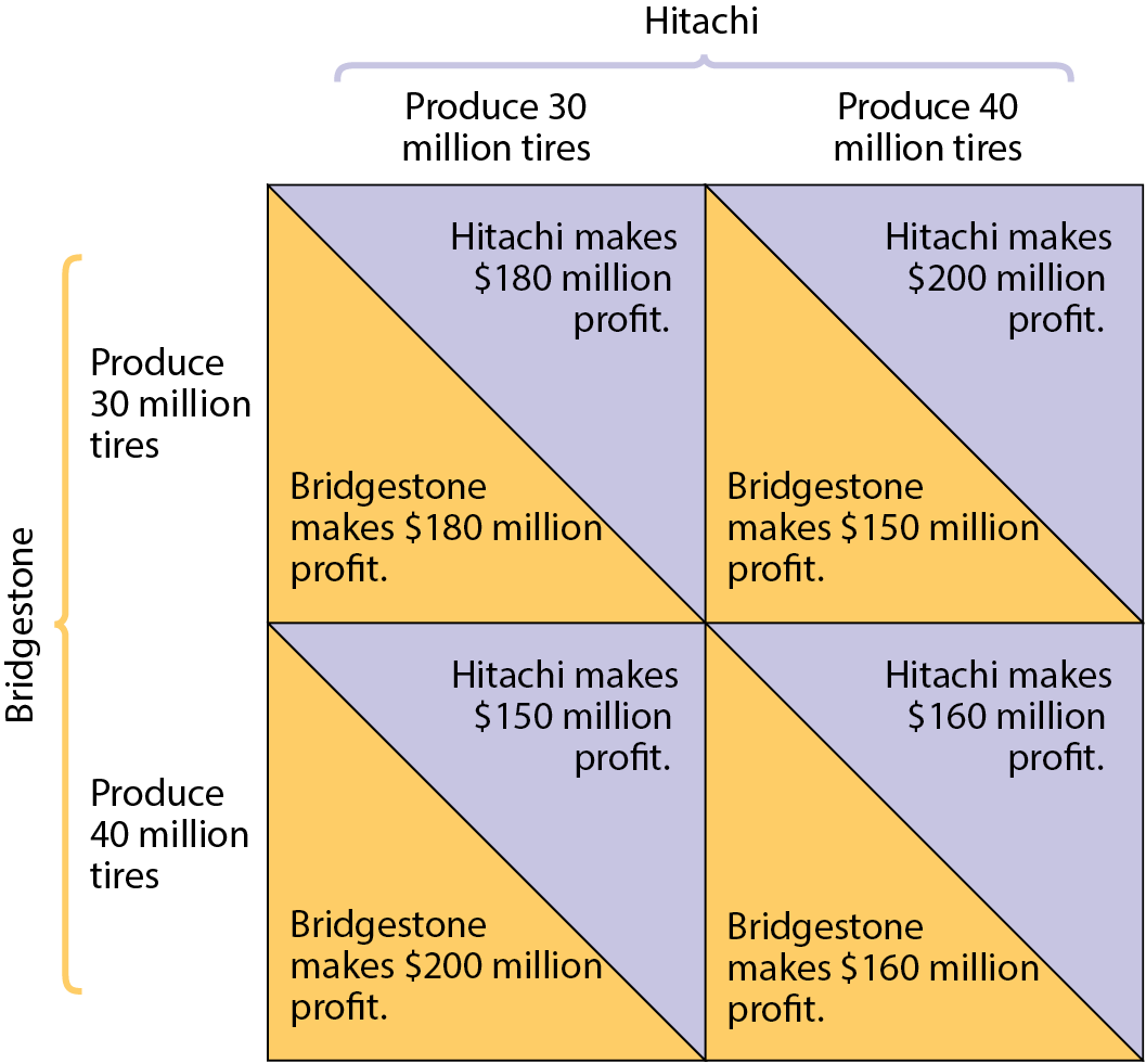
For inquiring minds: the arms race
Prisoners of the arms race:
Why did the United States and the Soviet Union spend so much money on (nonproductive) missiles and bombs during the Cold War?
Why did both sides fail to reach the best joint outcome: low military spending for both countries?
Overcoming the prisoners dilemma
Repeated interaction and tacit collusion
Players who don’t take their interdependence into account arrive at a Nash, or noncooperative, equilibrium.
But if a game is played repeatedly, players may engage in strategic behavior, sacrificing short-run profit to influence future behavior.
Tit for tat: a strategy of playing cooperatively at first, then doing whatever the other player did in the previous period.
How repeated interaction can support collusion
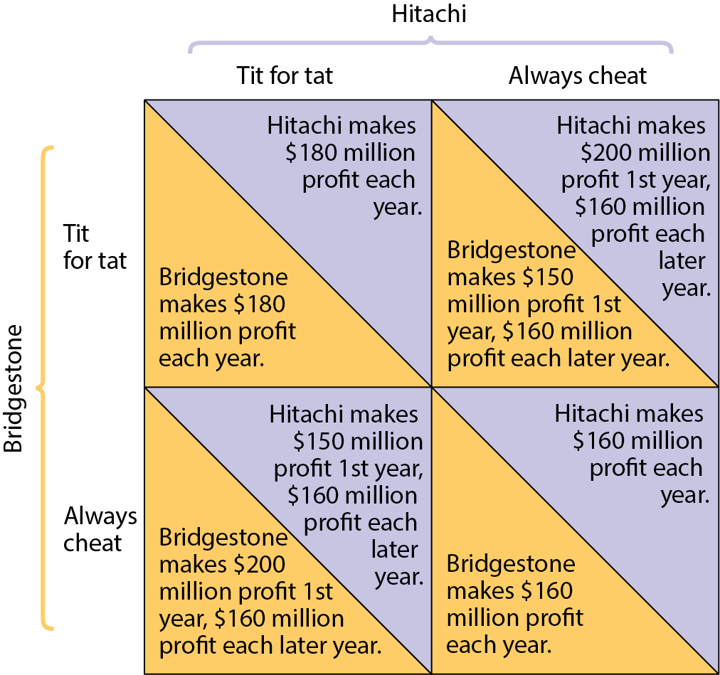
Economics in action: the ups and downs of the oil cartel
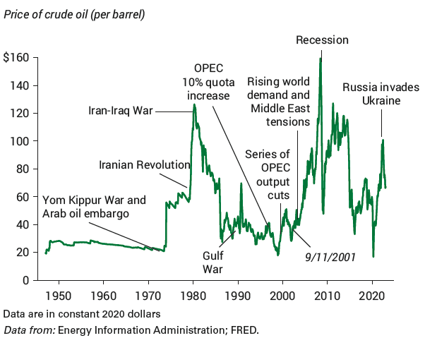
Oligopoly in practice: the legal framework
In the nineteenth century, when the growth of railroads created a national market, large firms emerged and formed cartels.
Many cartel members violated agreements and produced more.
In 1881, John D. Rockefeller’s Standard Oil Company came up with a solution to the cheating problem—trust.
The public backlash led to the Sherman Antitrust Act of 1890 and the ensuing antitrust policies.
Antitrust policies: efforts undertaken by the government to prevent oligopolistic industries from becoming or behaving like monopolies.
Oligopoly in practice: tact collusion
Many do succeed in achieving tacit collusion (unspoken agreements).
However, tacit collusion is limited by a number of factors, including:
less concentration.
complex products and pricing scheme.
differences in interests.
bargaining power of buyers.
Product differentation and price leadership
When collusion breaks down and prices collapse, there is a price war.
To limit competition, oligopolists often engage in product differentiation, an attempt by a firm to convince buyers that its product is different from the products of other firms in the industry.
In price leadership, one firm sets its price first, and other firms follow: one firm tacitly sets prices for the whole industry.
Firms that have a tacit agreement not to compete on price often engage in nonprice competition through advertising and other means instead.
How important is oligpoly
Given the prevalence of oligopoly, is the analysis of perfect competition still useful?
The answer is yes:
Even though many markets are oligopolistic, limits to collusion keep prices close to marginal costs—the markets behave almost as if they were perfectly competitive.
Predictions from supply and demand analysis are often valid for oligopolies.
The analysis of oligopoly is more difficult and messy than that of perfect competition. Keep in mind important issues, from antitrust policies to price wars, while trying to understand oligopolies
Chapter 18: Monolithic competition and product differentiation
What will we learn in this chapter?
What is monopolistic competition
Why do oligopolists and monopolistically competitive firms differentiate their products?
How are prices and profits determined in monopolistic competition in the short run and the long run?
How does monopolistic competition pose a trade-off between lower prices and greater product diversity?
What is the economic significance of advertising and brand names?
The meaning of monopolistic competition
Monopolistic competition is a market structure in which
there are many competing producers in an industry,
each producer sells a differentiated product, and
there is free entry into and exit from the industry in the long run.
Monopolistic competition is a little like monopoly and a little like perfect competition. Specifically, it has:
many competitors,
products similar but not identical, and
free entry into and exit from the industry in the long run.
Restaurants are monopolistic competitors.
Production differentiation
There are three important forms of product differentiation:
Differentiation by style or type
sedans versus SUVs (goods are substitutes but imperfect substitutes)
Differentiation by location
dry cleaner near home versus cheaper dry cleaner far away
Differentiation by quality
ordinary chocolate versus gourmet chocolate
There are two important features of industries with differentiated products.
Competition among sellers: Even though sellers are not offering identical goods, they are competing for a limited market. If more businesses enter the market, each will find that it sells less quantity at any given price.
Value in diversity: Consumers gain from the increased diversity of products.
Monopolistic competition in the short run
Same profit maximizing rule as previously used
Produce the Q at which MR = MC
Like monopoly firms, set price according to demand
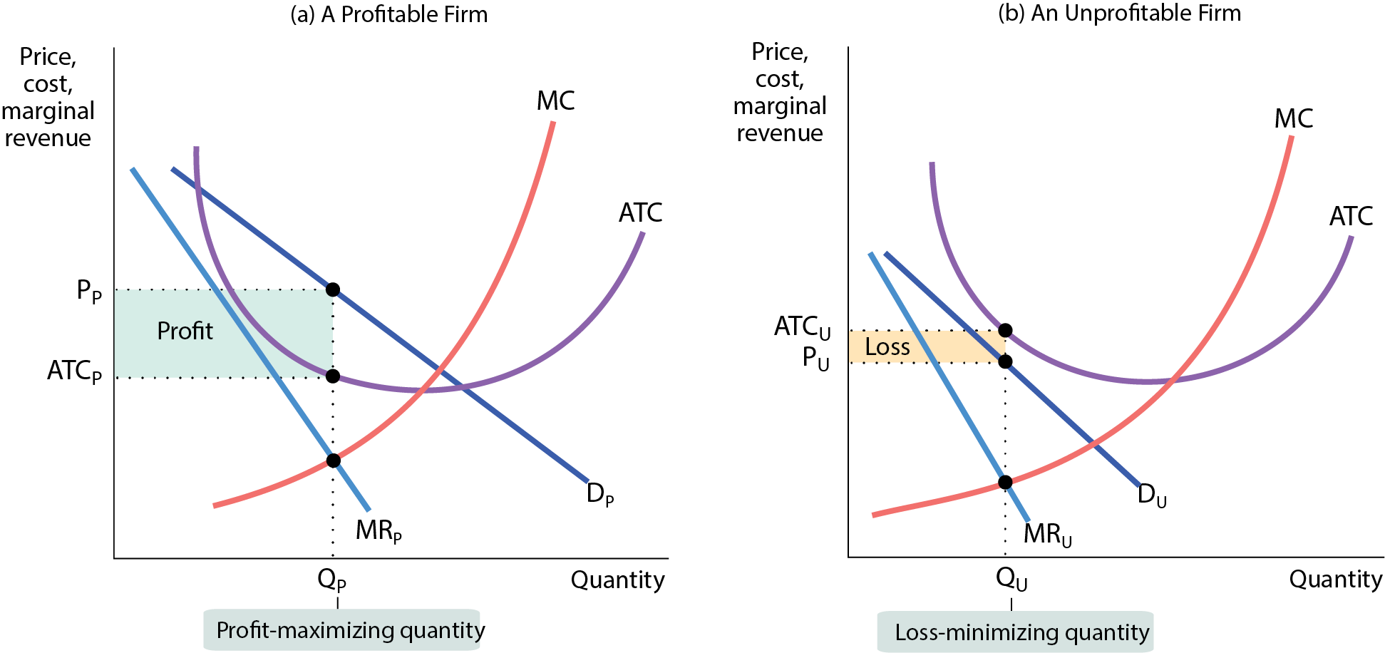
monopolistic competition in the long run
If existing firms earn profits, it will lead to the entry of new producers. New entrants mean fewer customers for the original firms: Demand and MR shift left.
When profits fall to zero, new entry stops.
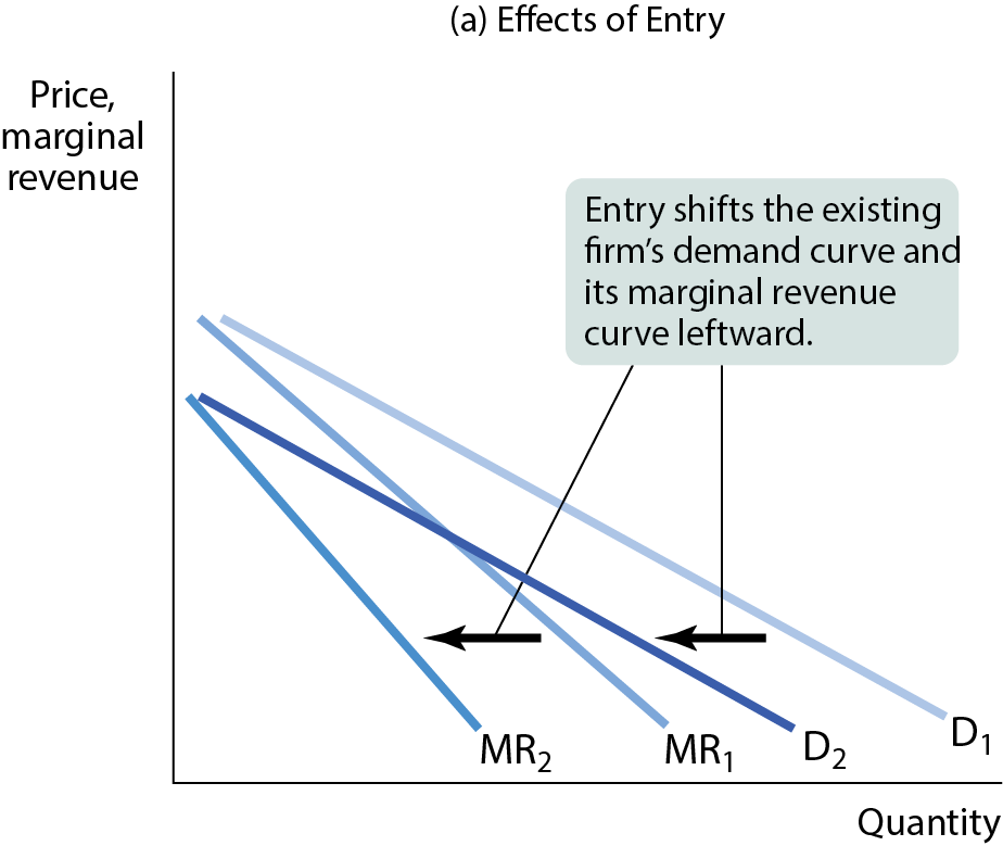
If existing firms lose money, some firms will exit the industry. The exit means more customers for the remaining firms: Demand and MR shift right.
When losses fall to zero, exit stops.
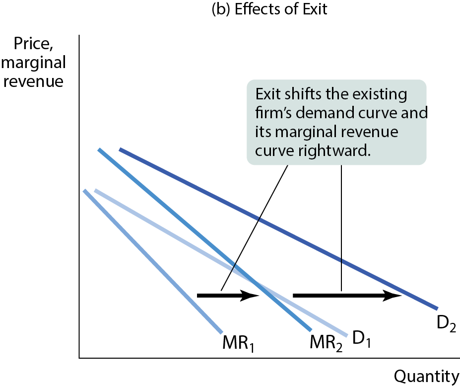
The long-run zero profit equilibrium
If firms are earning positive profits, new firms will want to enter the industry. This will reduce the demand curve facing each individual producer.
In the long run, each supplier will earn a zero profit, and price will equal ATC.
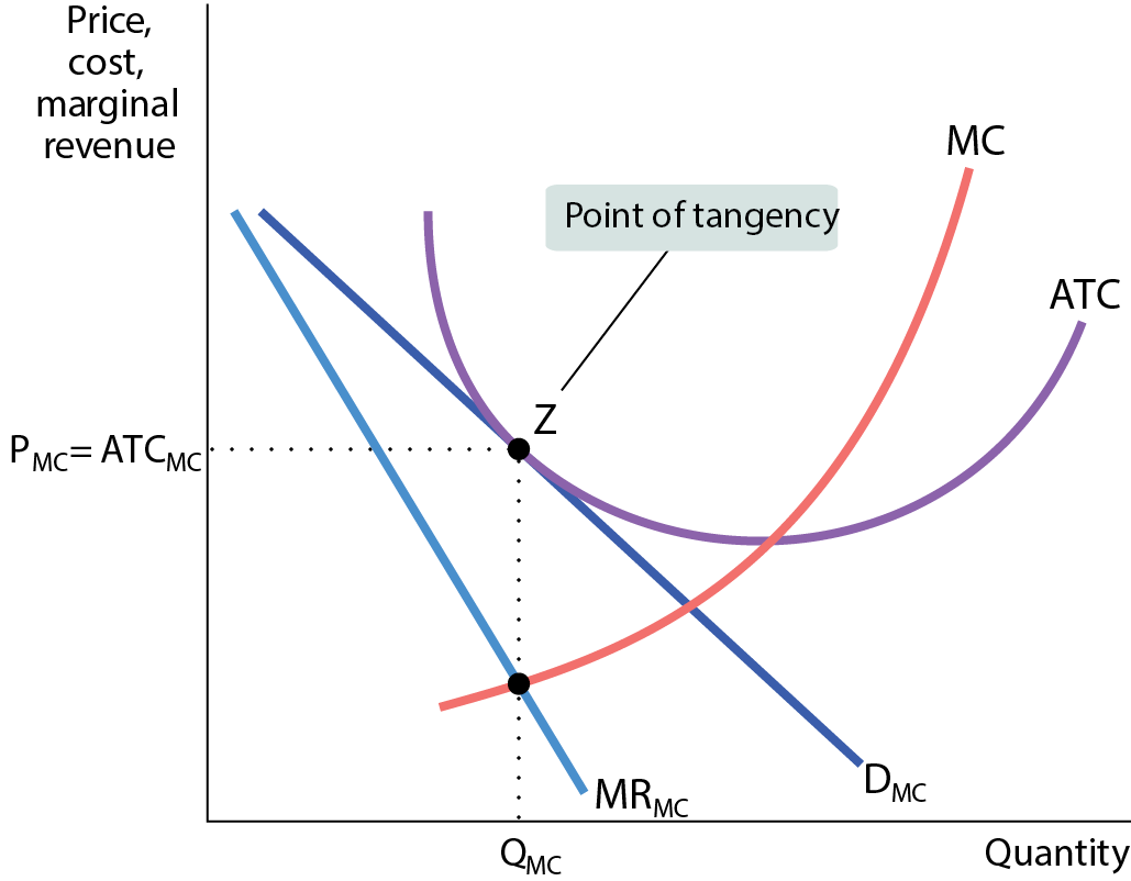
Monopolistic competition versus perfect competition
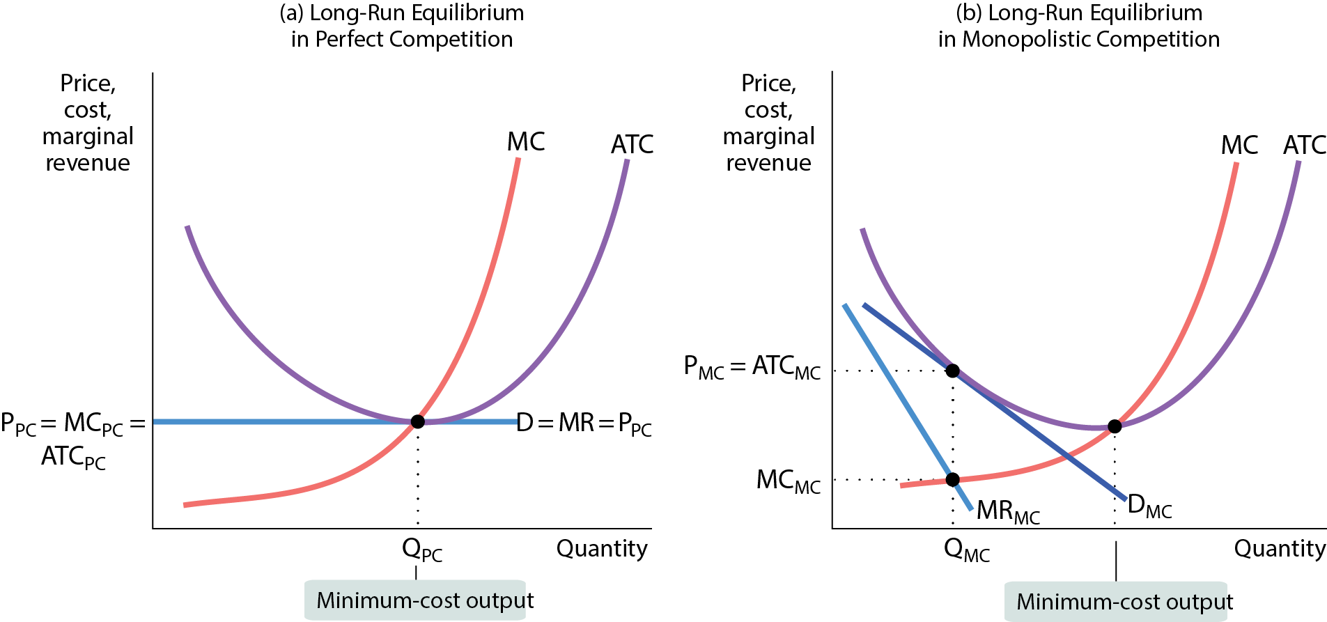
In panel (a), P = MC. In panel (b), P > MC
Monopolistic competitors, unlike perfect competitors, want to sell more at the going price. That’s why they engage in advertising that help increase sales.
In panel (a), the firm produces at the minimum of the ATC curve. In panel (b), the firm produces less than the quantity that would minimize average total cost, the excess capacity issue.
Is monopolistic competition inefficient
Inefficiencies of monopolistic competition:
A firm charges a price that is above marginal cost. As a result, some people are deterred from buying the product, and some mutually beneficial transactions go unexploited.
The excess capacity implies wasteful duplication because monopolistically competitive industries offer too many varieties.
Does that mean that monopolistic competition is inefficient? Not necessarily.
Diversity of products offered in a monopolistically competitive industry is beneficial to consumers.
There is a trade-off: more producers means higher average total costs but also greater product diversity.
Most economists now believe that duplication of effort and excess capacity in monopolistically competitive industries are not important issues in practice.
The economics of advertising
Oligopolies and monopolistically competitive firms advertise.
Is advertising good or bad? Both. (There are different types of advertising.)
Economies in action
THE PERFUME INDUSTRY: LEADING CONSUMERS BY THE NOSE
Only 3% of a perfume bottle’s cost is ingredients. The rest is marketing and packaging.
Studies show that people identify their favorite scents based on ego and branding, and often dislike the same scents in blind tests.
The role of advertising
The purpose of advertisements is to convince people to buy more of a seller’s product at the going price.
A perfectly competitive firm can sell as much as it likes at the going price and has no incentive to advertise.
A monopolistically competitive firm that charges a price above marginal cost can gain from advertising.
Is advertising a waste of resources?
Much of advertising informs potential buyers about what sellers have to offer.
Expensive ads serve as indirect signals conveying information about the quality of a firm’s products.
To the extent that advertising conveys important information, it is an economically productive activity.
Brand names
Do brand names create unnecessary market power, or do they serve a real purpose?
On one side, brand names often create unjustified market power.
On the other side, for many products the brand name does convey information about the quality of the product. They also offer some assurance that the seller is engaged in repeated interaction with customers and so has a reputation to protect.
Chapter 10: Externalities
What will we learn in this chapter?
What are externalities, and why do they lead to inefficiency and government intervention in the market?
How do negative externalities, positive externalities, and network externalities differ?
What is the Coase theorem, and how does it explain that private individuals can sometimes remedy externalities?
Why are some government policies to deal with externalities efficient while others are not?
Why are network externalities an important feature of high-tech industries?
Understanding externalities
An external cost is an uncompensated cost that an individual or firm imposes on others.
Examples of external costs:
air and water pollution
texting while driving
chemical runoff that affects fish stocks
External benefits are benefits that individuals or firms confer on others without receiving compensation.
Examples of external benefits:
beehives next to almond orchards
Education
preserved farmland
External costs and benefits are known as externalities.
External costs are negative externalities, and external benefits are positive externalities.
Externalities (spillovers): the impact on third parties of a transaction between others.
If fracking pollutes drinking water, it is a negative externality.
The costs and benefits of pollution
The marginal social cost of pollution is the additional cost imposed on society as a whole by an additional unit of pollution.
Acid rain, smog, contaminated water, etc.
The marginal social benefit of pollution is the additional gain to society as a whole from an additional unit of pollution.
Reducing pollution has an opportunity cost: It requires scarce resources that could have been used to produce other goods and services. The marginal social benefit of pollution is the goods and services that could be had by society if it tolerated another unit of pollution.
The socially optimal quantity of pollution is the quantity society would choose if all costs and benefits were fully accounted for.
Will a market economy, left to itself, arrive at the socially optimal quantity? No, it won’t.
The socially optimal quality of pollution
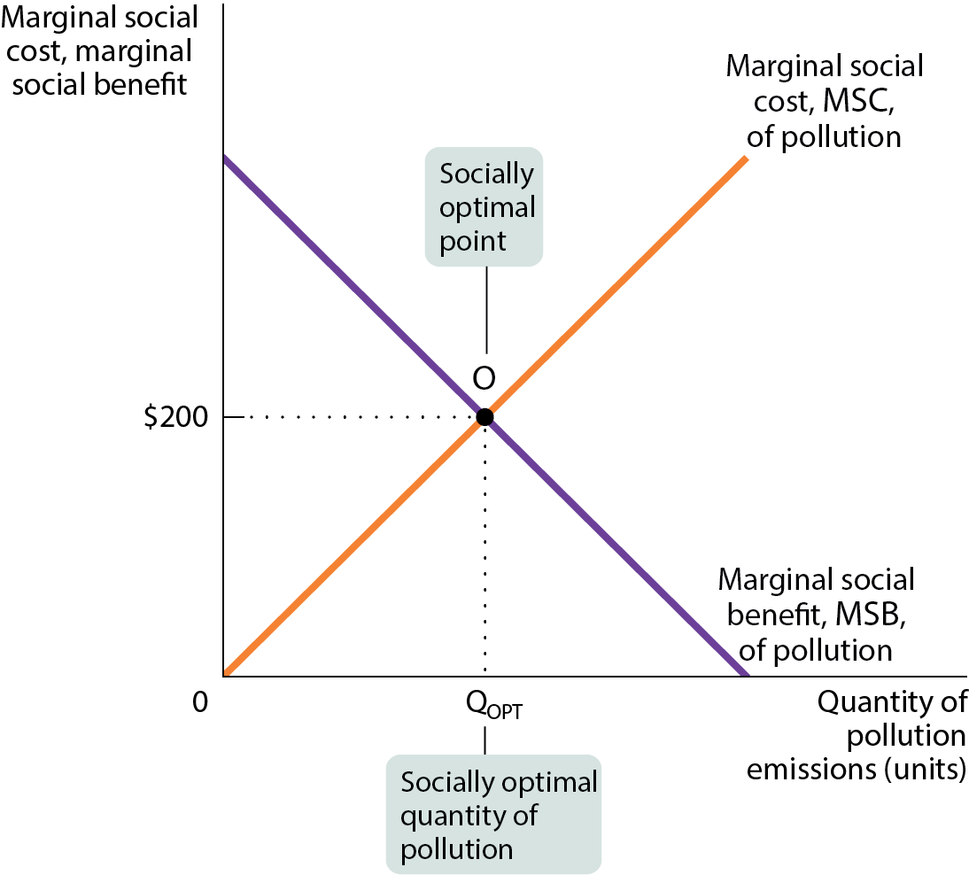
The socially optimal quantity of pollution isn’t zero.
It’s QOPT, where the marginal social benefit and marginal social cost are equal.
Why a market economy produces too much pollution
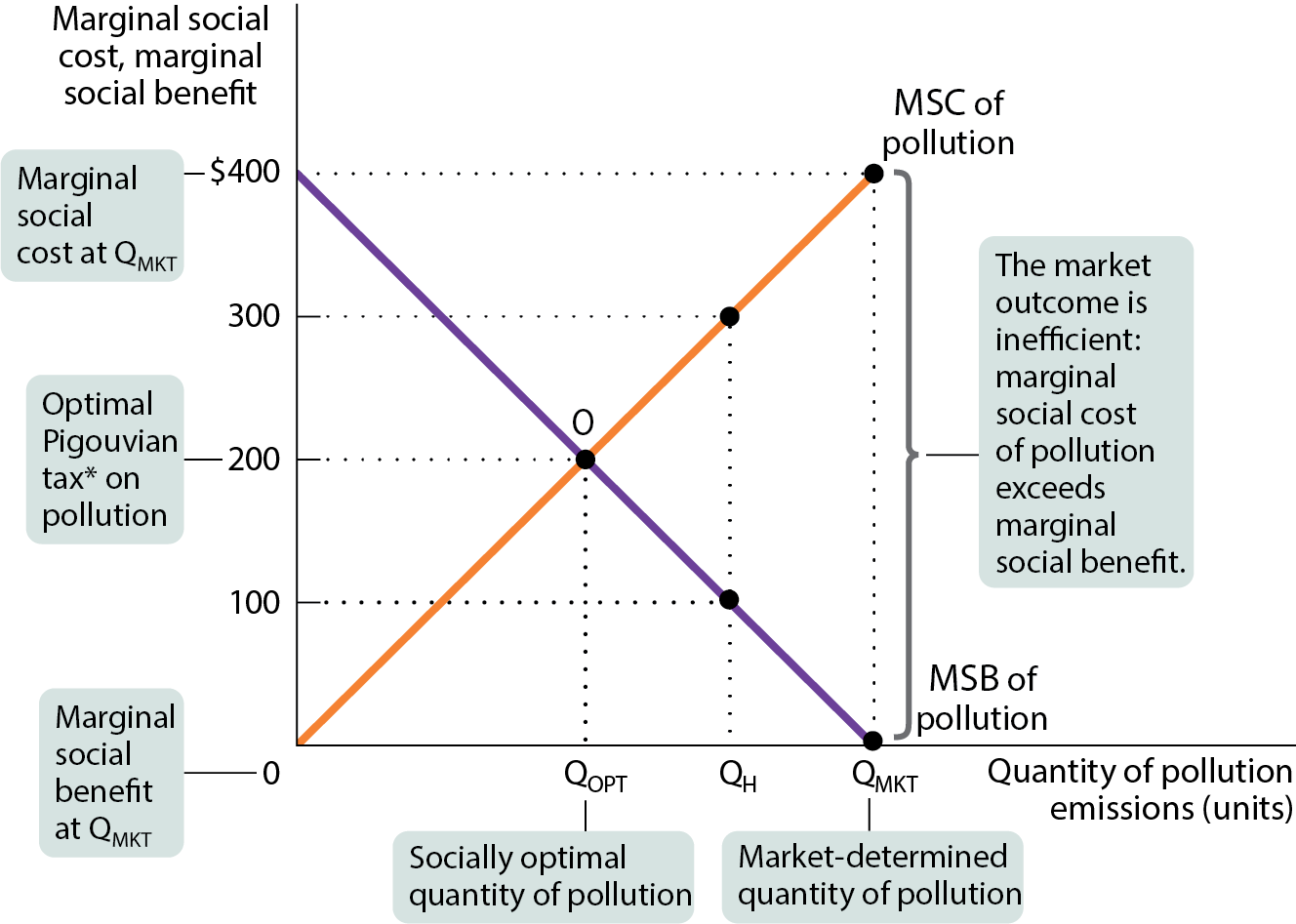
In a market economy without government intervention, polluters are the only ones who decide how much to pollute. They consider private benefits of pollution rather than social costs.
So instead of producing the socially optimal quantity, QOPT, they will produce QMKT.
At QMKT, the marginal social benefit of an additional unit of pollution is zero, while the marginal social cost of an additional unit is much higher.
Private solutions to externaility problems
Can the private sector solve the problem of externalities without government intervention?
The Coase theorem: The economy can reach an efficient solution, even in the presence of externalities, if the costs of making a deal are sufficiently low.
Example: a family agrees to stop playing loud music during their next-door neighbor child’s naptime in exchange for use of the lawnmower.
When individuals take externalities into account, they internalize the externality. In that case, the outcome is efficient without government intervention.
Why don’t private parties always internalize externalities? The problem is transaction costs—the costs of making a deal. They often prevent a mutually beneficial trade from occurring.
When those who are hurt by the externality are widely dispersed, cost of communication and negotiation is simply too high to achieve an efficient outcome.
Example: greenhouse gases.
When transaction costs prevent the private sector from dealing with externalities, it is time to look for government solutions.
Governemnt policies and pollution
If the market won’t solve its own externality problems, then what?
The three types of policies governments use to deal with pollution
environmental standards: rules that protect the environment by specifying actions by producers and consumers.
In the United States, the Environmental Protection Agency is the principal enforcer of environmental policies at the national level.
emissions taxes: cost depends on the amount of pollution a firm produces.
Pigouvian taxes: taxes designed to reduce external costs (example: an emissions tax designed to reduce coal production).
tradable emissions permits: licenses to emit limited quantities of pollutants; the licenses can be bought and sold by polluters.
Currently the largest emissions permit trading system is the European Union system for controlling emissions of carbon dioxide.
Comparing environmental policies
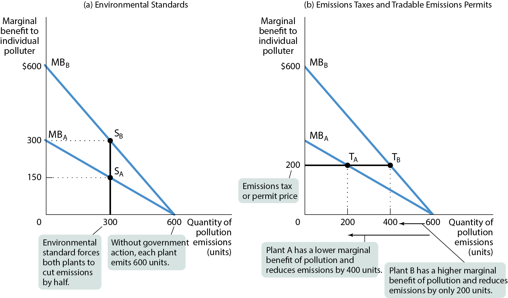
Two plants, A and B:
Plant A uses newer technology so that A’s marginal benefit curve lies below B’s marginal benefit curve.
An environmental standard requires both plants to cut emissions in half; this is inefficient, because it leaves the marginal benefit of pollution higher for B than for A.
An emissions tax as well as tradable permits achieve the same quantity of overall pollution efficiently.
Subsidies
Subsidies encourage polluters to switch from high-polluting activities to low-polluting activities.
For example, the Inflation Reduction Act (IRA) of 2022 gives a $7,500 tax credit for the purchase of an electric vehicle for qualifying buyers.
Cap and trade
Since 1994, the United States has had an SO2 cap-and-trade system, and acid rain has been reduced by 94% from 1994 to 2022—relatively cheaply.
In 2005, the first cap and trade system for trading greenhouse gases—called carbon trading—was launched in the European Union. Nearly two decades later, carbon trading has grown rapidly around the world. In 2021, approximately $850 billion in permits were traded globally.
The economies of climate change
Climate change is the human-made change in Earth’s climate from the accumulation of greenhouse gases caused by the use of fossil fuels.
Greenhouse gases are gases that trap heat in Earth’s atmosphere.
The causes of climate change
Fossil fuel is fuel derived from fossil sources such as coal and oil.
Renewable energy sources are energy sources that are inexhaustible, unlike fossil fuel sources, which are exhaustible.
Clean energy sources are energy sources that do not emit greenhouse gases. Renewable energy sources are also clean energy sources.
World energy consumption remains overwhelmingly dependent upon fossil fuels. In 2021, they accounted for approximately 83.4% of total consumption, renewables accounted for only 12.6%, and nuclear energy accounted for approximately 4%.
Policies to address climate change
Government subsidies to R&D: Since the 1980s, the U.S. government has provided billions of dollars in subsidies for R&D dedicated to lowering the cost of clean energy sources.
Multilateral agreements: They set common objectives and allocate burden-sharing across countries. In 2015, 196 countries signed the Paris Agreement, with a common goal of limiting the increase in the Earth’s temperature to 2° centigrade.
Climate change mitigation
Are the costs of addressing climate change too high?
Global losses from runaway climate change are estimated at 20% of GDP by 2100.
4.6 million people die annually from air pollution caused by burning fossil fuels.
The health benefits of switching to clean energy is estimated to be 5% of global GDP.
In 2019, more than 3,500 economists advocated for a carbon tax to fight climate change.
The economies of positive externalities
Sometimes a market includes benefits that bystanders receive.
External benefit: a benefit received by people other than the consumers or producers trading in the market
Do motorcycle riders provide an external benefit to those waiting for an organ transplant?
Positive externalities are the mirror images of negative externalities.
Left on its own, the market will produce too little of a good that generates external benefits.
But society as a whole is better off when policies are adopted that increase the supply of such a good.
Why a market economy preserves too little farmland
Without government intervention, the quantity of preserved farmland will be zero. (See Figure 6.)
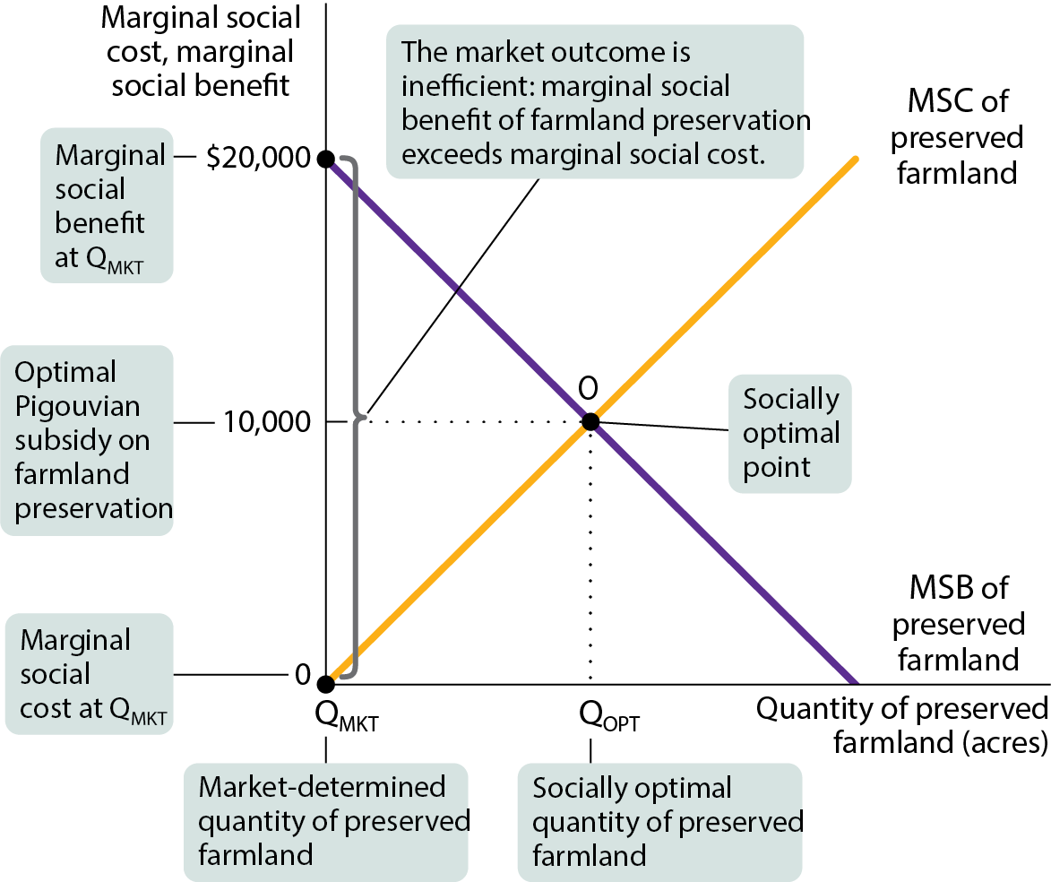
At the socially optimal point O, the marginal social cost equals the marginal social benefit, and QOPT acres of farmland are preserved.
The market alone will preserve zero acres of farmland, QMKT.
Because farmers bear the entire cost of preservation but gain none of the benefits, they will preserve an inefficiently low quantity of acres.
How can the economy produce the socially optimal QOPT? Use a Pigouvian subsidy, the payment designed to encourage activities that generate positive externalities.
Pigouvian subsidy
A Pigouvian subsidy: a payment designed to encourage activities that yield external benefits.
The socially optimal quantity can be achieved by a Pigouvian subsidy equal to the marginal social benefit at the optimal quantity.
Positive externalities in today’s economy
The single most important source of positive externalities is the creation and spreading of knowledge, known as a technology spillover.
A technology spillover is a positive externality that results from knowledge spread among individuals and firms.
illegal
One of the best-known research clusters is the Research Triangle in North Carolina, anchored by several universities, hospitals, and companies such as IBM, Pfizer, and Qualcomm.
Network externalities
A good is subject to a network externality when the value of the good to an individual is greater when a large number of other people also use the good.
Examples include:
Communication systems such as telephones, telegraphs, fax machines
Railway systems
Hub-and-spoke air travel
A good is subject to positive feedback, also known as a bandwagon effect, when success breeds greater success and failure breeds failure.
The more popular Windows is, the more software is made for it and the more popular it becomes.
Chapter 11: Public goods and common resources
What will we learn in this chapter?
What is a public good, and how is it different from a private good?
What is a common resource, and why is it overused?
What is an artificially scarce good, and why is it underconsumed?
Why do markets typically fail to supply these types of goods efficiently?
How can government intervention make society better off in the production and consumption of these types of goods?
Characteristics of goods
Excludable: People who don’t pay can be easily prevented from using a good.
Example: jeans
Rival in consumption: The same unit of the good cannot be consumed by more than one person at a time (or at all).
Example: cheeseburger
Your Happy Meal: both excludable and rival.
Nonexcludable: People who don’t pay cannot be easily prevented from using a good.
Example: national defense
Nonrival: More than one person can consume the same unit of the good at the same time.
Example: digital music
Asteroid deflection is both nonexcludable and nonrival.
Four types of goods
Private goods are excludable and rival in consumption, like wheat.
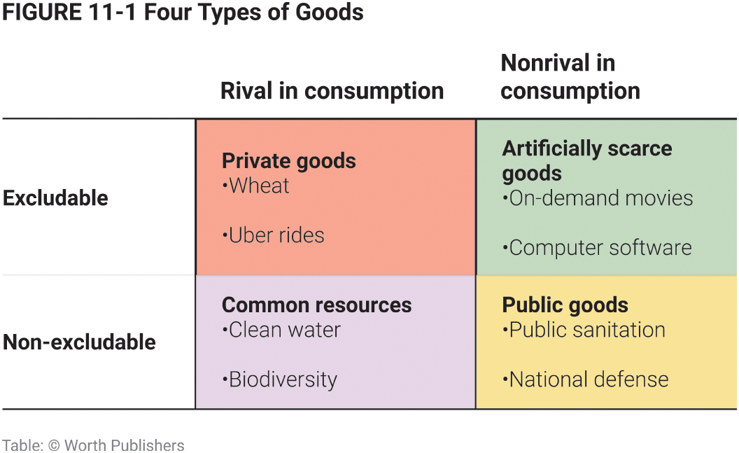
Public goods are nonexcludable and nonrival in consumption, like a public sewer system.
Common resources are goods that are nonexcludable but rival in consumption, like water in a river.
Artificially scarce goods are excludable but nonrival in consumption, like on-demand movies on Amazon Prime.
Why markets can supply only private goods efficiently
Markets cannot supply goods and services efficiently unless they are private goods—excludable and rival in consumption.
Nonexcludable goods have the free-rider problem: many individuals are unwilling to pay for consumption of nonexcludable goods and instead will take a “free ride” on anyone who does pay.
Example: in a student group project, shirkers free ride on someone else’s effort.
Nonexcludable goods suffer from inefficiently low production—they are undersupplied.
Goods that are excludable and nonrival in consumption suffer from inefficiently low consumption—they are underconsumed.
Example: Amazon Prime has a marginal cost of zero but charges $4 per movie so that viewers will only consume movies up to the point where their marginal benefit is $4 instead of zero.
Public goods
A public good is a good that is both nonexcludable and nonrival in consumption.
Examples: disease prevention, defense, scientific research.
Because these goods are nonexcludable, they suffer from the free-rider problem, so no private firm would be willing to produce them.
And because they are nonrival in consumption, it would be inefficient to charge people for consuming them.
Society must find nonmarket methods for providing these goods.
Providing public goods
Public goods are provided through a variety of means:
Voluntary contributions (example: private donations for scientific research);
Individuals or firms who make money in an indirect way (example: meta supplies social media platforms—almost entirely supported by advertising);
Social encouragement or pressure in small communities (example: volunteer fire departments);
The government (most important public goods—national defense, the legal system, disease control, and so on—are provided by government and paid for by taxes).
How much of a public good should be provided
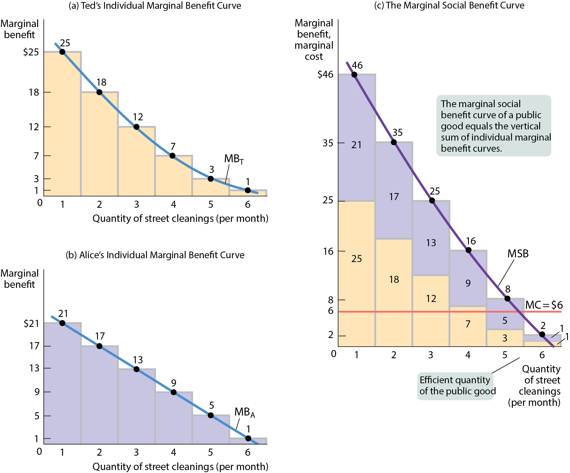
If the government provides the public good, how much should it produce?
Produce the quantity where marginal social benefit of a public good equals marginal cost of producing it.
The marginal social benefit of a public good is equal to the sum of the individual marginal benefits enjoyed by all consumers (the sum of each consumer’s willingness to pay for that unit).
Imagine a city with two residents, Theo and Abby. Assume that Theo and Abby truthfully tell the government their willingness to pay for another unit of the public good—they tell the government their marginal benefits.
The efficient quantity of a public good is the quantity at which the marginal social benefit is equal to the marginal cost of providing it.
The marginal social benefit of one more unit of a public good is always greater than the individual marginal benefit. That is why no individual is willing to pay for the efficient quantity of the good.
The problem of providing public goods is similar to the problem of positive externalities: there is a market failure that calls for government intervention.
Residents could and would vote to tax themselves to pay for provision of public goods.
Cost benefit analysis
It’s straightforward to estimate the cost of supplying a public good.
Estimating the benefit is harder because governments can’t just ask people their willingness to pay for it (their individual marginal benefit).
For example, if street cleaning were scheduled according to the stated wishes of homeowners, the streets would be cleaned every day—an inefficient level of provision.
If governments relied on the public’s statements when deciding how much of a public good to provide, they would likely provide too much. In contrast, relying on voting has problems as well—and is likely to lead to too little of the public good being provided.
Common resources
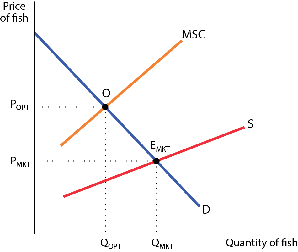
A common resource is nonexcludable and rival in consumption.
They tend to be overused if left to the market: individuals ignore the fact that their use depletes the amount of the resource remaining for others.
When one person catches a fish, there are fewer fish available for everyone else.
Each person has the incentive to fish before others.
In an unregulated market, the quantity of the common resource used, QMKT, exceeds the efficient quantity, QOPT.
The efficient use and maintenance of a common resource
Because common resources pose problems similar to those created by negative externalities, the solutions are also similar:
Tax or regulate the use of the common resource.
Create a system of tradable licenses for the right to use the common resource.
Make it excludable and assign property rights to it.
A Pigouvian tax can reduce the use of a common resource to the efficient quantity. For example, when visitors to national parks pay a fee, the number of visitors falls.
Create a system of tradable licenses: The policy maker issues the number of licenses that corresponds to the efficient level of use of the good. Example: individual transferable quotas, or ITQs, help reverse the collapse of fisheries because each ITQ holder has a financial interest in the long-term maintenance of his fishery.
The most natural solution is to assign property rights: Make the good excludable and assign property rights over it to someone. The owner then will have an incentive to protect the good.
Artifically scarce goods
An artificially scarce good is a good that is excludable but nonrival in consumption.
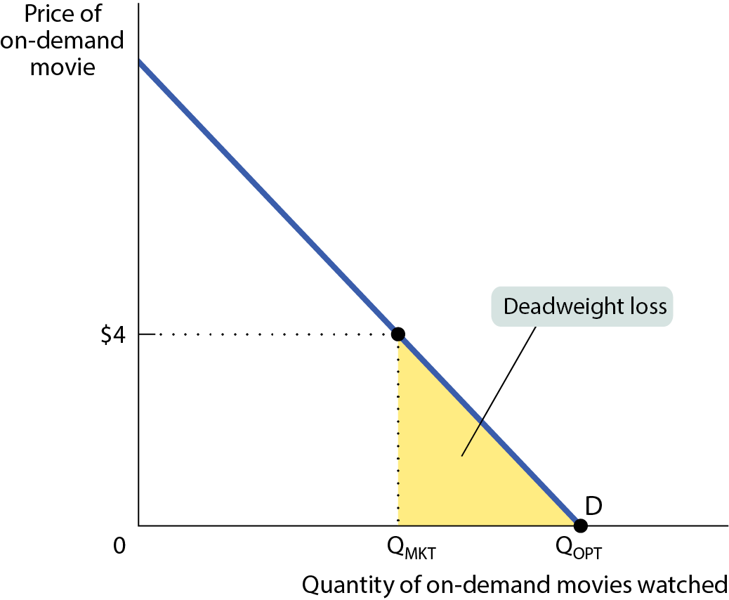
Example: on-demand movies.
The marginal cost of allowing one more person to consume the good is zero.
However, because it is excludable, sellers charge a positive price, which leads to inefficiently low consumption.
The problems of artificially scarce goods are similar to those posed by a natural monopoly.