The z Table and Hypothesis Testing with z Tests
The z Table
Overview of the z Table
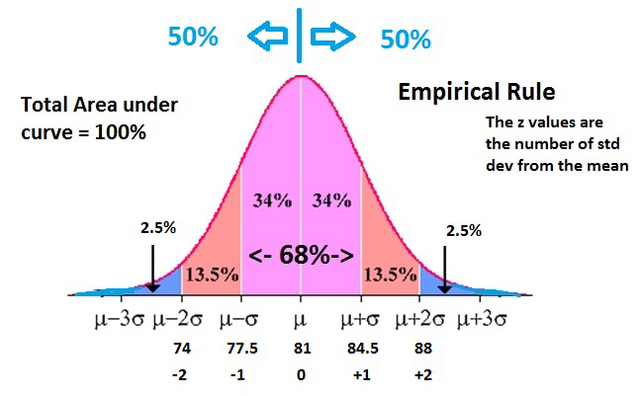
In Chapter 6, the empirical rule was introduced:
About 68% of scores fall within one z-score of the mean.
About 96% of scores fall within two z-scores of the mean.
Nearly all scores fall within three z-scores of the mean.
These are useful guidelines, but for precise calculations, the z-table is used.
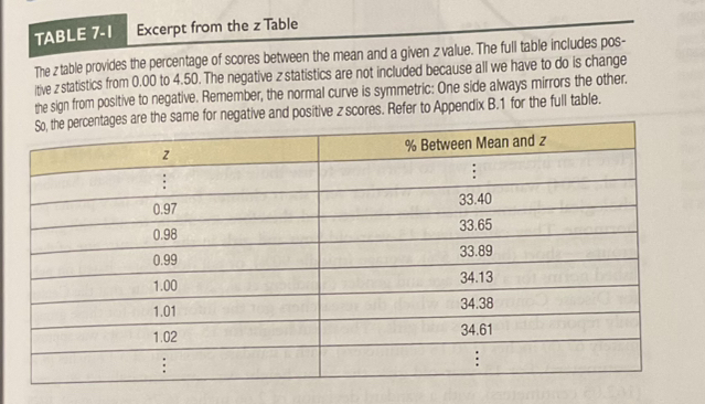
The full z table is located in Appendix B.1, with an excerpt provided in Table 7-1.
Understanding the Z Table
The z table gives percentages of scores between the mean and a given z value.
Negative z-statistics can be calculated by changing the sign of their positive counterparts.
The normal curve is symmetric, implying that the percentages associated with negative and positive z scores are identical.
Example Table Excerpt (Table 7-1)
Raw Scores, z Scores, and Percentages
Relationship Between Scores
Much like various names can refer to the same individual (e.g., "Christy," "Tina" for "Christina"), z scores, raw scores, and percentile rankings refer to the same statistical concept.
The z table facilitates the transition between these types of scores.
It serves as a mechanism for stating and testing hypotheses by standardizing different observations onto a common scale.
Calculating Percentages with the z Table
Step 1: Convert the raw score into a z score.
Step 2: Use the z table to find the percentage of scores between the mean and the calculated z score.
Note: The z scores in the table are typically positive; negative z scores can be deduced using the symmetry of the normal distribution.
Visual Representation of the Standardized z Distribution
The z table allows for the calculation of percentages above and below a specific z score.
Symmetry of the normal curve informs us that negative z scores mirror their positive counterparts, providing identical percentages.
Example Calculations
Example 7.1
A research team investigated whether shorter children experience poorer psychological adjustment compared to taller peers, potentially justifying treatment with growth hormone (Sandberg et al., 2004).
Methodology
The study categorized boys and girls aged 15 years based on height into three classifications:
Short (bottom 5%)
Average (middle 90%)
Tall (top 5%)
Data acquired from the Centers for Disease Control provided average heights for 15-year-old boys and girls.
Boys:
Mean height: 67.00 inches (170.18 cm)
Standard deviation: 3.19 inches (8.10 cm)
Girls:
Mean height: 63.80 inches (162.05 cm)
Standard deviation: 2.66 inches (6.76 cm)
Case of Jessica
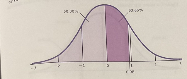
Step 1: Convert Jessica's height (66.41 inches) to a z score using girls' data:
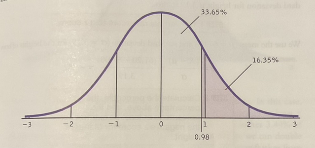
Step 2: Search for z = 0.98 in the z table, yielding a percentage of 33.65% between the mean and Jessica's z score.
Derived Percentages
Jessica's Percentile Rank:
Total percentage below Jessica: 50% (scores below the mean) + 33.65% = 83.65%
2.) Percentage of Scores Above Jessica:
Above scores: 50% (total above mean) - 33.65% = 16.35%
3.) Scores as Extreme as Jessica's:
Total extreme scores in both directions: 16.35% + 16.35% = 32.70%
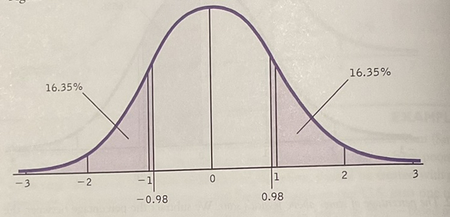
Classification:
Since 16.35% of 15-year-old girls are taller than Jessica, she is not in the top 5%, so we can classify her as being average in height.
Example 7.2
Case of Manuel (Height: 61.20 inches)
Steps to Analyze Manuel's Height
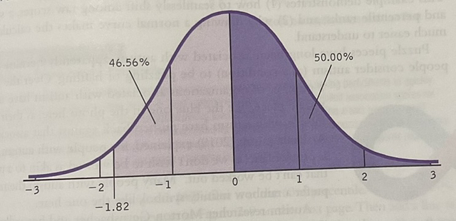
Step 1: Convert his height to a z score using the boys' data:
Step 2: Identify z = 1.82 in the z table, yielding 46.56% percentage between the mean and z.
Derived Percentages for Manuel
Manuel's Percentile:
Score below: 50% - 46.56% = 3.44%
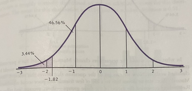
2.) Percentage of Scores Above Manuel score :
Above scores: 50% + 46.56% = 96.56%
3.) Extreme Percentages:
Total extreme heights: 3.44% (below) + 3.44% (above) = 6.88%
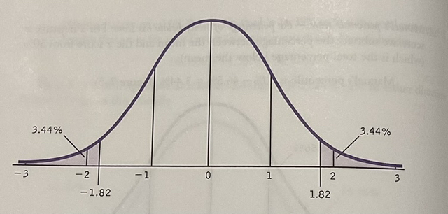
Classification:
Manuel's percentile rank of 3.44% places him in the lowest 5% of heights, categorizing him as short.
Example 7.3
Exploration of the Relationship between Raw Scores, z Scores, and Percentiles
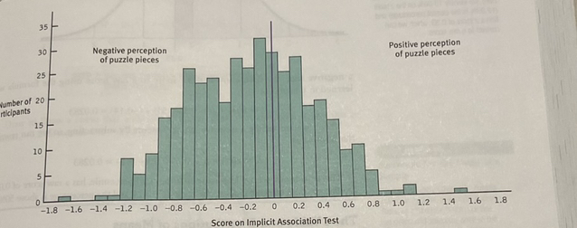
A symbolic representation of autism using a puzzle piece has elicited criticism from individuals with autism who prefer a rainbow infinity symbol (Jessop, 2019).
A study aimed to assess negative perceptions linked to the puzzle piece among the general public (Gernsbacher et al., 2018).
An Implicit Association Test (IAT) revealed a normal distribution of implicit association scores towards puzzle pieces, where the mean was -0.14, and the standard deviation was 0.51, indicating a negative bias across the sample.
Calculating a Participant's IAT Score at the 63rd Percentile
Determine Raw Score:
The score measures above the mean since 63% is greater than 50%.
Calculate percentage: 63% - 50% = 13%.
Locate 12.93% in the z table, yielding a z score = 0.33.
Convert z Score to Raw Score:
Using the formula:
Substituting in numbers:
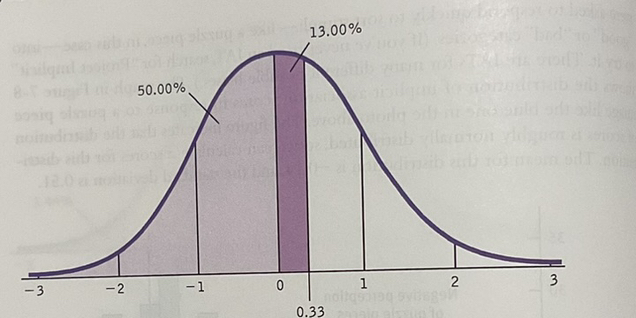
Result Validation
The calculated score corresponds correctly as above the mean and aligns with the percentile rank being above 50%.
Conclusion
The document demonstrates the utility of the z table for hypothesis testing through systematic steps, examples involving real-world applications, and explicit calculations.
Future studies could expand on the application of z-scores to other psychological metrics, enhancing the understanding of height influences and perceptions across different demographics.