BAR Summary

B1

• Supply and Demand curve: supply goes up with quantity & price, demand goes down with price.

  

B2

M1 - Capital Structure (CS)

debt vs equity, how company funds itself

WACC - Weighted Average Cost of Capital

• LOWEST WACC = BEST Value for firm & best CS

• WACC Formula: (A)* (B) *(C)

        A. ((Cost of Stock %) * Proportion of CS that is Stock )

        B. ((Cost of Preferred Stock%) * Proportion of CS that is Preferred Stock )

        C. ((Cost of Debt %) * Proportion of CS that is Debt)

Cost of Retained Earnings

• How much a firm should grow to keep stockholders happy (otherwise stockholders = mad and take money away)

• Market risk premium = market return rate - risk free rate

3 Methods to calculate “Expected Return of Investment” (for investor) or “Cost of Retained Earnings” (for company):

#1. CAPM - Capital asset pricing model

• Cost of equity = Risk-free rate + Beta * Market Risk Premium

• Beta of investments = % change in price / % change in market

#2. DCF: Discounted Cash Flow

• [Cash flow / Market value price per stock] x Growth Rate

#3. BYRP: Bond Yield plus Risk Premium

• Market Risk Premium + Pretax cost of long term debt.

Analyzing Capital Structure

• Loan covenant - requirements from lenders to secure debt. Positive debt covenants ensure you maintain certain levels or ratios. Negative debt covenants restrict you from doing things.

• Retention - Increase in RE / Net Income. AKA- portion of income not paid out in dividends.

• Growth Rate - (Return on Assets x Retention) / [1 - (Return on Assets x Retention)]

• High Financial leverage - when there’s less owners so existing owners get more profits → less equity + more debt CS = more EBIT to cover interest

• Operating Leverage - when company has less variable costs → higher contribution margin.

• Levered firm - company that has debt in its CS. unlevered = all equity no debt. levered firm can deduct interest on debt from taxes = good.

M2 - Working Capital

How businesses use cash, collect cash, and manage payments to get the most return on capital.

• Net working capital = current liabilities - current assets

AR Management

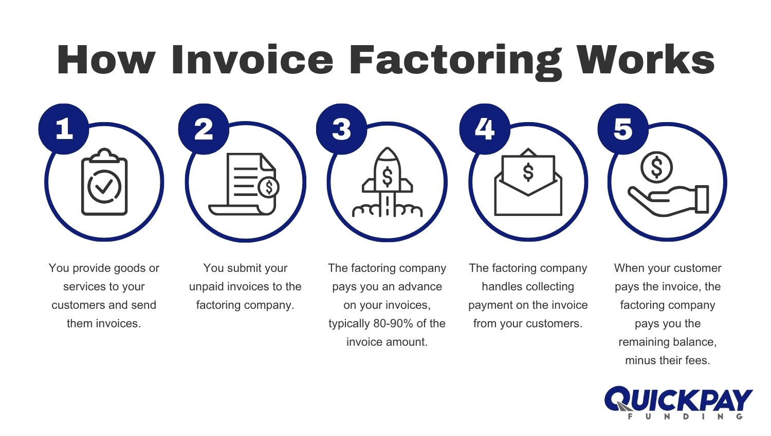
• Factoring - a company gives you a % of your AR $$ now in exchange for a fee and interest payments. You get benefit of money now instead of waiting and less administrative work. Con = expensive.

Inventory Management

• Reorder point = safety stock + (sales during lead time)

• Economic Order Quantity = SQUARE ROOT of [(2 * Annual Sales * Cost to place each order)/ Annual carrying cost per unit]

  • Make sure that the time measure (like annual/quarterly/weekly all match up).

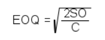
• Order size gets larger as "S" or "O" gets bigger (numerator) or as "C" gets smaller (denominator).

• SCOR - Supply Chain Operations Reference Model. Plan, Source, Make, Deliver.

• 3 types of Inventory Management Issues:

  1. Just in time - order gets placed → manufacture starts → gets to customer = less lag & more efficient

     • JIT is a pull-through inventory system, as the customer's order drives the need for inventory.

     • Push systems begin with forecasting customer demand.

  2. Kanban - “hit me over the head with a can” → OOPS we ran out = order more.

  3. Computerized - computer tells when to order more when stock is running low.

AP Management

• Annual Cost of NOT taking a cash payment discount =

  • Effective Interest on Missed Discount Rate x Cycles of days of delayed payment per year

    • another way to look at it is…

  • [Forgone discount % / (100% - Foregone Discount %)] x [360 / (Pay period - Discount period)]

• Short-term financing - debt that matures <1 yr

  • Pros: faster conversion of operating cycle, lower interest rates.

  • Cons: higher interest rate risk from fluctuating market/economy, credit worthiness can be affected impacting future funding for capital.

• Long-term financing - debt that matures >1 yr. pros and cons are opposite of short term financing.

M3 - Valuation

Methods to value stocks & equity

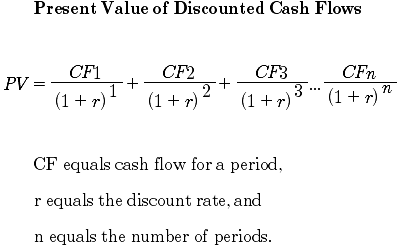
• Absolute Value Models: Assigns an intrinsic value to an investment by calculating the PV of the cash flow.

• Relative Valuation Model: Uses price multiples, (financial ratios) to determine if the stock is undervalued, fairly valued, or overvalued.

Types of absolute value calculations:

• Annuities: same cash flow each period for certain time period.

  • Annuity Due = beginning of period

  • Ordinary annuity = end of period

• Perpetuities (aka Zero Growth Stock): same cash flow forever = like a dividend.

  • Present value of a perpetuity = the stock price.

  • Stock price = Dividends / Required Rate of Return %

• Constant (Gordon) Growth Dividend Discount Model (DDM): assumes dividend will grow at same rate every year.

  • Present value (aka: price at specified period)

    

  • Get the required rate of return from the CAPM

  • higher dividends → higher value

• Discounted Cash Flow Analysis:

  1. Dividend discount model (DDM) - expected dividends = basis for PV of future CF

  2. Free cash flow model (FCFF) - available cash after covering working capital needs = basis for PV of future CF

Types of relative valuation calculations:

1. Price Earnings (P/E) Ratio = Stock Price / Earnings per Share for 1 Fiscal Year

   • PE Ratio x Earnings for 1 year = Current stock price

     • Forward vs Trailing P/E Ratio:

       • Forward = future earnings & future EPS.

       • Trailing = past earnings & past EPS

   • high P/E → growth expectations

   • low P/E → undervalued or risky

2. PEG Ratio: P/E/G → the lower the better

3. Price-to-Sales Ratio: more stables than PE Ratios

4. Price-to-Cash-Flow Ratio: price per share / cash flow per common shares outstanding

   • A metric showing how much the market pays for each $1 of projected cash flow. A P/CF of 15 means each $1 of next year’s cash flow is valued at 15 times.

5. Price-to-Book Ratio: price per share / common stockholders’ equity per common shares outstanding

Options

• Option: contract where a person can buy or sell a stock (or other asset) at a specific price within a certain period of time. American option → exercised any time. European option → exercised at maturity.

  • Buy → call option (the stock sings: “call me maybe!”)

  • Sell → put option (the stock says: “put me down!”)

• The Black-Scholes Model: option value now; price, time, volatility, interest rate. Assumes a constant risk-free interest rate over the option's term in the calculation

• Binomial (Cox-Ross-Rubinstein) Model: option value over time; price, steps, up/down, probabilities

Debt

• Bonds pay interest (coupons) each period

• Then return principal at the end

• To calculate price of a bond:

  • Discount each coupon payment

  • Discount the final principal

  • Add them all up

Fair Value

• Hierarchy of inputs: ranking of valuation inputs by reliability (Level 1–3).

  • Level 1 = quoted price for item.

  • Level 2 = comparable item’s price.

  • Level 3 = estimates, not observable price.

• Fair value measurement: if principal market exists (market where most units is sold), then FV = value in principal market. if no principal market, then FV = most advantageous.

• Market, income, cost approach: ways to value asset.

  • Market = comparables

  • Income = present value cash flows

  • Cost= replacement cost

M4 - Financial Decision Models

• Cash Flows: Direct = actual cash; Indirect = adjusts NI → cash; both → same net CF

• Asset Disposal: Sell old asset → gain/loss affects taxes → impacts CF → use after-tax proceeds = SP – tax on gain

• Depreciation: non-cash but saves taxes → tax shield = Dep × tax rate → treat as cash inflow

NPV steps: PV cash savings/inflows = PV net cash outflows

1. Initial Investment (first yr when buying t=0): purchase + install + WC → always negative

2. Operating CF: savings/revenues are taxable → use after-tax CF = inflow × (1 – tax rate)

3. Salvage value: after tax gain/loss from last yr

4. NPV: Initial investment (which is negative) - PV inflows → NPV > 0 accept, < 0 reject

• Ask:
  👉 “Is this ONE payment or MANY?”

• Pick:

  • one payment → “PV of $1”

  • many → annuity

• THEN multiply

• Discounting: PV factor = FV / (1+r)^n; time=0 = no discount

• Profitability Index: PI = PV inflows / initial → >1 accept

• IRR (internal rate of return): rate where NPV = 0 → IRR > hurdle → accept

  • tells us “related interest rate”

• Payback method: initial investment / annual CF → liquidity focus, ignores time value

  • Discounted Payback (BET): same but uses PV

• EVA (economic value added): after-tax income (excluding interest expense) – (Required return)

  • Required return = Investment * WACC.

  • positive = accept

M5 - Marginal Analysis

• Marginal analysis = only include costs/revenues that change; ignore sunk costs, include opportunity costs.

  • Opportunity cost is the potential benefit lost by selecting a particular course of action. If the land is developed rather than sold, the potential selling price foregone is an opportunity cost.

    • the next best use of productive capacity.

  • Sunk costs are costs incurred in the past that will not change as a result of any decision made in the future. These costs are considered irrelevant in marginal analysis decisions because they do not change.

• Special order: if extra capacity → accept if price > variable cost; if full → include opportunity cost.

• Make vs buy: choose lower relevant (avoidable) cost.

• Sell or process further: process if incremental revenue > incremental cost.

• Keep or drop: keep if lost contribution margin > avoidable fixed costs.

B3

M1 - Cost Accounting

• Prime cost = Direct materials + Direct labor

• Conversion cost = Direct labor + Manufacturing overhead

• Overhead cost: all indirect costs to manufacturing a product. there is fixed overhead which is going to be there regardless and there is variable overhead which can increase your indirect costs based on how much you produce.

• Relevant range = range where cost behavior assumptions hold
  → Outside it, fixed costs may change and cost formulas break

• Job order costing = customized products/projects (each job tracked separately)

  • Ex: building a custom house

• Process costing = mass production (use averages across units)

  • Ex: making identical bottles of soda

• Equivalent units = % complete units expressed as full units

  • Used to allocate costs between completed units & ending WIP

  • Ex: 100 units at 50% completion = 50 full units

• FIFO vs Weighted Avg

  • FIFO = current period costs only. Ex: only this year’s production costs

  • WA = mix of beginning + current costs. Ex: blends last year’s + this year’s (like mixing batches)

• ABC (Activity-Based Costing)

  • Allocates overhead based on actual activities (cost drivers)

  • More accurate than traditional because it matches cost → cause

    • Ex: if product uses more machine setups → gets more overhead

• Direct vs Step-down (support allocation)

  • Direct = ignores support-to-support services

    • Ex: HR costs production only (ignores any IT costs helping HR)

  • Step-down = partially accounts (one-way allocation)

    • Ex: IT → HR → production (one direction)

• Joint product costing

  • Costs incurred before split-off point

  • Allocate joint costs based on relative sales value (usually)