Antagonists

Forms of Antagonism:

Receptor Antagonism:

• Most common and specific form of antagonism.

• Antagonist binds to receptor → prevents agonist from activating it.

• Mechanisms:

  • Competitive: Competes directly with agonist at the binding site.

  • Non-competitive: Binds at allosteric site or blocks receptor function.
    
    

Physiological Antagonism:

• Occurs when two agonists act on different receptors to produce opposing physiological effects.

• Overall effect = partial or complete cancellation of each other’s actions.

  • Example:

    • Noradrenaline → ↑ heart rate via β₁-adrenoceptors

    • Acetylcholine → ↓ heart rate via M2 muscarinic receptors
      
      

❗No direct receptor blockade; effects are due to opposing physiological pathways.

Chemical Antagonism:

• Antagonist binds directly to the agonist, forming an inactive complex.

• Prevents agonist from reaching its receptor.

• Does not require receptor binding by antagonist.

  • Example:

    • Protamine (positive) binds heparin (negative), which blocks the anticoagulant effect.
      
      

Antagonism of the Stimulating Messenger:

• Antagonist inhibits the endogenous stimulating agent before receptor binding.

• Often involves antibodies or binding proteins.

  • Example:

    • Avastin (bevacizumab) binds VEGF, which prevents receptor activation. This then blocks tumour angiogenesis.

Types of Receptor Antagonists:

Competitive Antagonists:

• Bind same active site as the agonist.

  • Can be reversible or irreversible.

    • Effect: Prevent agonist binding; can be overcome by increasing agonist concentration. It is surmountable.
      
      

Sub-Types:

• Reversible:

  • Non-covalent, transient binding

    • Equilibrium exists → agonist can outcompete

      • Surmountable: maximum effect can still be reached

• Irreversible:

  • Covalent or very strong bond

    • Permanent blockade → reduces number of functional receptors

      • Example: Phenoxybenzamine inactivates α-adrenoceptors which leads to sustained sympathetic inhibition

Non-Competitive Antagonists:

• Bind allosteric site or block receptor function (e.g., ion channels).

• Effect not dependent on agonist concentration.

  • Mechanisms:

    • Allosteric modulation leads to a conformational change, which decreases agonist efficacy.

    • Pore blockade in ion channels prevents ion flow.

• Example: Memantine is an NMDA receptor which reduces neuronal excitation.

Mechanisms of Action:

Competitive Antagonists:

• Bind same site → directly block agonist.

  • Concentration-response curves:

    • Rightward shift → higher agonist concentration needed

    • Maximum response unchanged (Rmax) if enough agonist added

• Example: Propranolol shifts formoterol (β-agonist) dose-response curve rightward.

Non-Competitive Antagonists:

• Bind allosteric site or block function → reduce receptor efficacy.

  • Concentration-response curves:

    • Decreased maximum response (Rmax)

    • EC50 usually unchanged

• Advantageous when endogenous agonist levels are high.

Concentration Response Curves for Competitive Antagonists:

• Reversible competitive antagonists:

  • Rightward shift of agonist dose-response curve

  • Maximum response (Rmax) can still be reached

• Example: Formoterol (β-agonist) + propranolol (β-blocker) → rightward shift in airway smooth muscle relaxation curve.

Non-Surmountable Antagonism:

• Maximum response cannot be reached, regardless of agonist.

• Mechanisms:

  • Irreversible antagonism: Covalent binding reduces receptor population

    • Example: Phenoxybenzamine leads to a permanent α-blockade.

  • Non-competitive antagonism: Allosteric binding or pore block reduces receptor efficacy

    • Example: Navarixin is a CXCR2 non-competitive antagonist, and has anti-inflammatory & anti-tumour properties.

Implications for Drug Development:

• Therapeutic versatility:

  • Non-competitive antagonists reduce overstimulation, independent of agonist levels

  • Useful in diseases with high endogenous agonist activity

• Economic considerations:

  • Complex molecules (antibodies) are effective but costly

    • Example: Avastin £21,000 per patient for six weeks → higher dose vs. macular degeneration

Functional Gaddum and Schild Analyses:

Conditions Required:

1. Reversible, Competitive Antagonism

   • The antagonist must compete directly with the agonist for the same receptor binding site.

   • Binding must be rapid, reversible, and at equilibrium.

   • The antagonist should not cause receptor conformational change or affect the response pathway itself.

2. Equilibrium Conditions

   • Measurements must be taken under steady-state conditions where agonist-antagonist-receptor interactions are stable.

3. Single Receptor Population

   • The response should be mediated by a single receptor type.

   • Mixed receptor types or multiple signalling pathways invalidate the analysis.

4. Surmountable Antagonism

   • Increasing the concentration of the agonist should overcome the antagonist’s effect.

     • A parallel rightward shift in the concentration–response curve without change in the maximum response (R_max).

5. Stable and Linear Agonist-Response Relationship

   • The tissue or system should produce a consistent and proportional response to receptor activation.

     • The agonist and antagonist must reach steady-state concentrations in the tissue.

Only when these conditions are met can accurate estimates of KB, pKB, and pA2 be obtained.

— — — — —

The Gaddum equation describes the quantitative relationship between the agonist and antagonist concentrations needed to produce the same level of response:

$\frac{[A]}{[A']} - 1 = \frac{[B]}{K_B}$

Where:

• [A] = agonist concentration producing a specific response (without antagonist).

• [A'] = agonist concentration producing the same response (with antagonist present).

• [B] = antagonist concentration.

• KB = equilibrium dissociation constant of the antagonist (affinity measure).

— — — — —

The dose ratio (r) is defined as:

$r = \frac{[A']}{[A]}$

Substituting into the Gaddum equation gives:

$r-1=\frac{[B]}{K_B}$

When [B] = K_B​, then r = 2. Effectively, the antagonist concentration that doubles the agonist concentration required to produce the same effect.

— — — — —

Antagonist Affinity (pA₂ and pK_B)

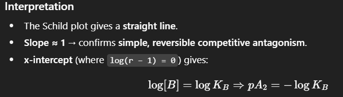
• pA₂ ​= −logK_B​.

  • Thus:

    • Higher pA₂ = higher affinity of the antagonist.

    • If the Schild slope = 1, then pA₂ = pK_B​.

— — — — —

The Schild analysis provides a graphical determination of antagonist affinity.

1. Measure agonist EC50 values in the presence of several antagonist concentrations.

2. Calculate the dose ratio (r):         $r = \frac{EC50_{\text{(with antagonist)}}}{EC50_{\text{(control)}}}$

   3. Apply the Schild equation: log (r−1) = log[B] − logK_B.

   4. Plot log (r-1) (y-axis) vs. log[B] (x-axis).