GEOG352 FINAL REVIEW
learning objectives
identify the need for spatial interpolation
define spatial tessellation methods for interpolation
define approximation interpolation methods
lecture 10
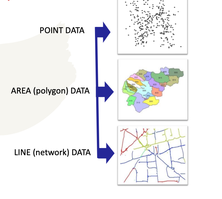
point values in 2 dimension is (x,y)
point values in 3 dimension is (x,y,z)
3rd dimension is the attribute value
Defining spatial interpolation
analysis of spatially continuous data: focus on understanding the spatial distribution of values of one single attribute over an entire study region
main goal of spatial interpolation: estimate the values for the entire study area based on the measured attribute values of existing sample points
done by
1. finding a function or a model that appoximate/estimate the mising values then
2. predicting/estimating the values at points where the attribute has not been sampled
the spatial interpolation problem:
given a sest of spatial data in the form of points (or areas), spatial interpolation is the process of finding the function that will estimate or predict values for any other points (or areas) and will best represent the whole surface
spatial interpolation: mathematical process of finding a function that will estimate/predict unknown attrubute values at any point from a given set of sample point locations
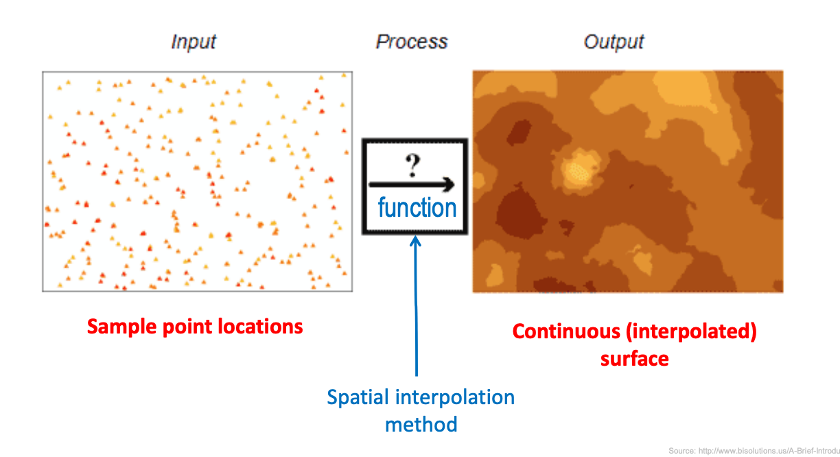
spatial interpolation methods take into consideration locations of sample points denoted with coordinates (x,y) and the attribute values (z)
ex: elevation, depth, pollution level, temp, soil propoerty, etc..)
the continuous surface: defined as a feature which contains continuous information about estimated z attribute values across a given study area
spatial interpolation methods should not be applied if the attributes of sample points represent the presence of an event (crime/disease), people, or some physical phenomenon (volcanoes, buildings), as the created continuous surface will be meaningless
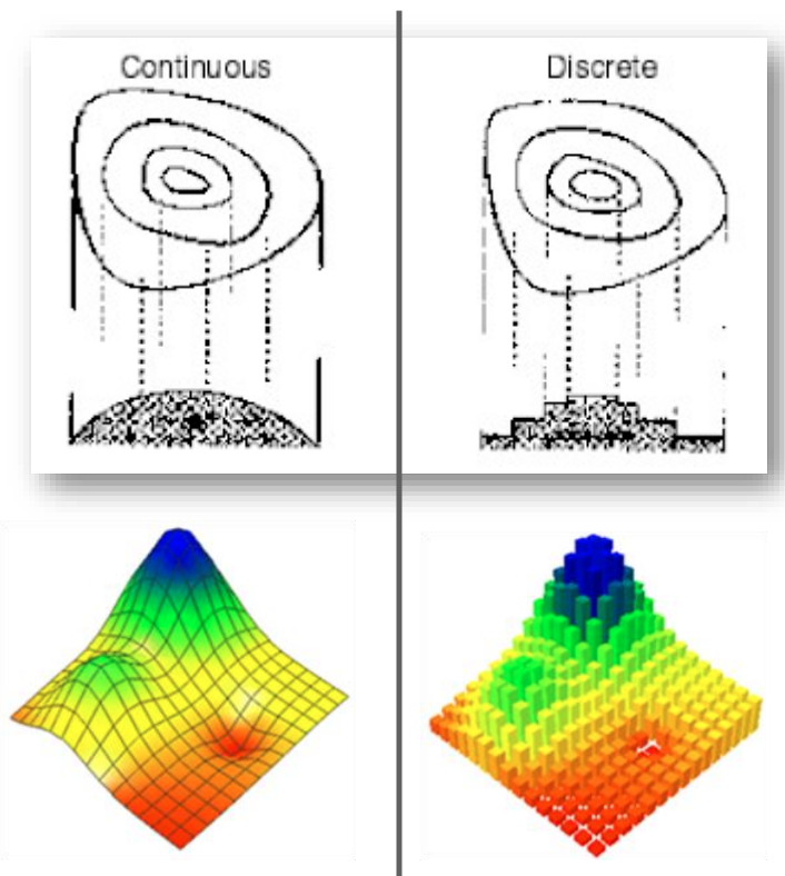
type of interpolation surfaces
continuous: statistical surfaces where data occurs at every possible location in the study area
possible to obtain a measurement for any point anywhere in the area (elevation, air temp)
discrete: statistical surfaces where data is limited to selected areas are are mostly suitable for qualitative (nominal) data
all locations (entire surface) within the area around the data point have the same value (population by census)
dsicrete surfaces with very small areas (areas of very small spatial resolution) are often considered as continuous surfaces)
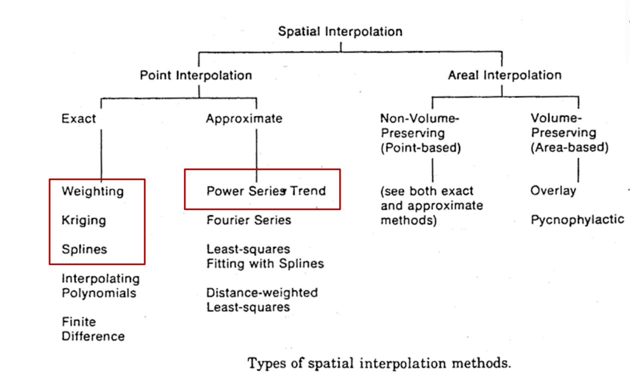
methods of spatial interpolation for point data
for discrete surfaces
spatial tessllation
vonoi diagrams and delaunay triangulation
for continuous surfaces
approximate spatial interpolation method
trend surface analysis
exact spatial interpolation methods
spline, inverse distance weighted method, kriging
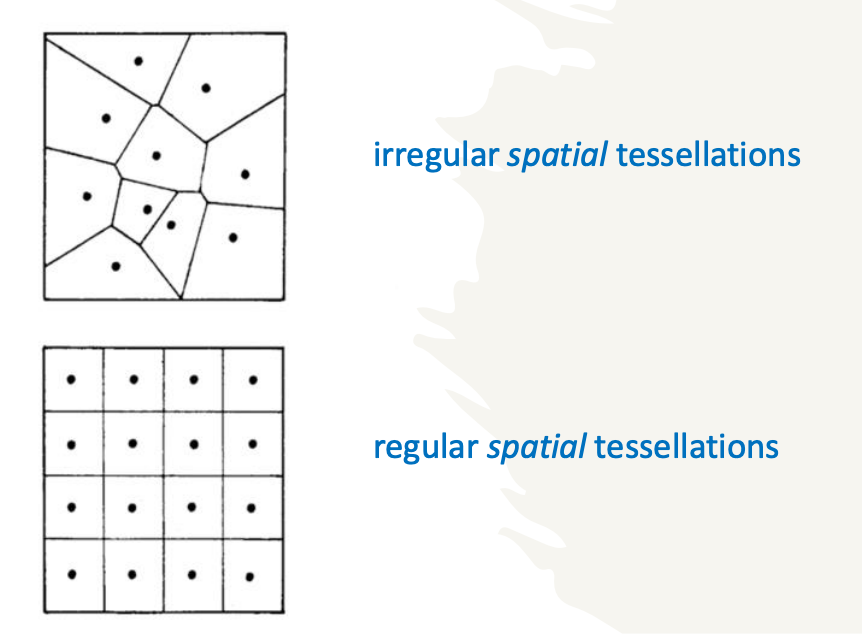
spatial tessellation methods
objective is to divide and delineate landscape/study area by creating boundaries of new polygons - discrete surfaces
for the given sample points, the boundary is to be derived from the nearest data points
tessellation polygons divide a surface or a study region in a way that is determined by the configuration of locations of the data points
irregularly spaced: resulting polygons/areas are of irregular shape
regularly spaced: resulting polygons/areas are equal to the grid/regular spacing
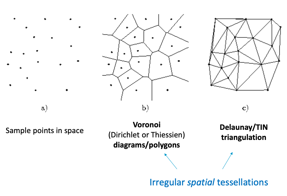

each point (a-j) will define a region in the Voronoi diagram
each polygon encloses all locations that are closer to one particular point than to any other.
highlighted triangle and bisectors illustrate the construction of a voronoi vertex where three or more edges meet
delaunay triangle
triangle is equilateral as possible - no other points lie inside the circle
build digital terrain surface/visibility analysis
advantages and disadvantages of spatial tessellation methods
the computation of irregular tessellation methods are well known algorithms and there are mathematical discussions
the interpolated surface within each diagram/tessellation will have the same value, so errors cannot be calculated and the computation of a value at an unsampeld point becomes a problem
adding or removing a point will require redesigning the entire tessellation structure
the edges of the study area tessellation structures have weird shapes
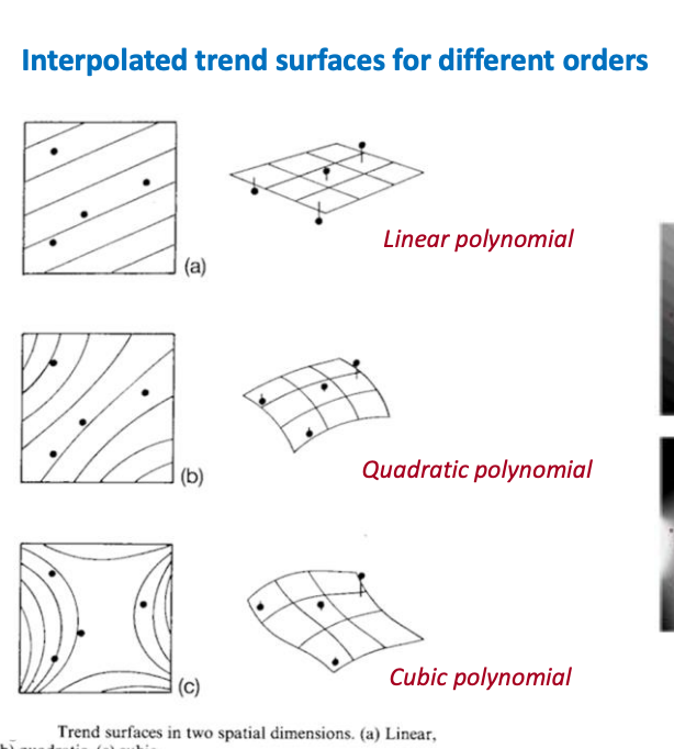
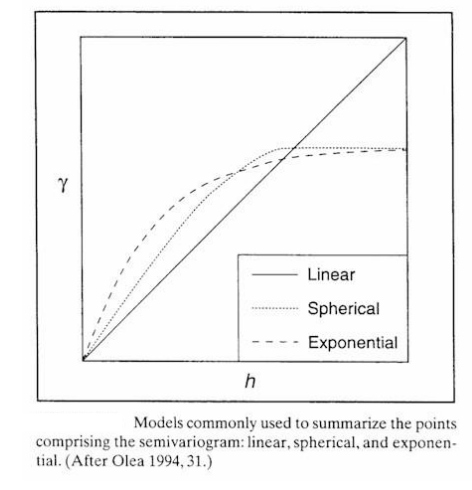
approximate spatial interpolation methods
trend surface analysis: approximative method to derive continuous surface by using a low order polynomial or trigonometric function
fitted between the sample data points
parameters are estimated using the least squares method - minimize the total difference b/w the original surface and the polynomial function

a straight line fit minimizes vertical distances (Errors) from each data points to the line
a polynomial better fits the ups and downs and represents a more complex spatial trend, capturing variations that are not linear
advantages and disadvantages of trend surface interpolation
the trend surface method generates the broad range models of low-order surfaces
the statistical significance of trend surface interpolation can be tested by using the tecniques of analysis of variance b/w the trend and the residuals from the trend
this method becomes increasingly difficult to describe a physical meaning of obtained surfaces when higher polynomials are used
this is a smoothig technique, rarely passing through original sampling data points so it is often used as exploratory method for the data prior to application of some other exact interpolation technique
learning objectives
identify the need for spatial interpolation
define splines and inverse distance weighting interpolations
define kriging interpolations
lecture 11
exact spatial interpolation methods
points that are closer together on the ground are more likely to have similar values of a property than ponts further apart (first law of geog)
spatial interpolation proceeds by finding the function that will permit fitting a surface model to the measure sample data points, and then the values at any desired locations can be estimated/predicted using the spatial interpolation method
spline interpolation method
general purpose interpolation method that fits a minimum curvature through input points (sample points)
conceptually - the same as bending a rubber sheet through all the points while minimizing the total curvature of the surface
a mathematical function is fitted to a specified number of nearest sampling points while passing through all the sample points
linear, quadratic, cubic spline
least square spline
minimum curvature spline
linear spline: uses linear functions
n=1, degree of freedom=0
a set of line segments that simply connect the known values of the function at sample points
quadratic spline uses quadratic functions
n=2, degree of freedom=1
sensitivity: if one point is slightly moved, the curve changes in four intervals — moving one point affects a large portion of the spline, not entirely local
cubic spline: cubic functions
n=3, degree of freedom=2
with sharp corners: splines naturally round corners, need extra points to fix shape
highorder splines affect more of the curve
breakpoint locations affect whether the spline honours data points or smooths over them
advantages and disadvntages of spline interpolation
splines are piecewise functions using few points at a time, the interpolation can be quickly calculated
splines retain small scale features, are aesthetically pleasing and can produce quick and clear spatial overview of the data
cubic splines provide the most natural and smooth surface found in the real world while linear or quadratic splines do not generate smooth surfaces
problem with using splines is that different results will be obtained with choosing different break/sample points or when using a different number of sample points
there is no direct estimates of the errors assocaited with spline interpolation
trend surface vs spline interpolation
both methods aim to predict values between known points, but use different strategies
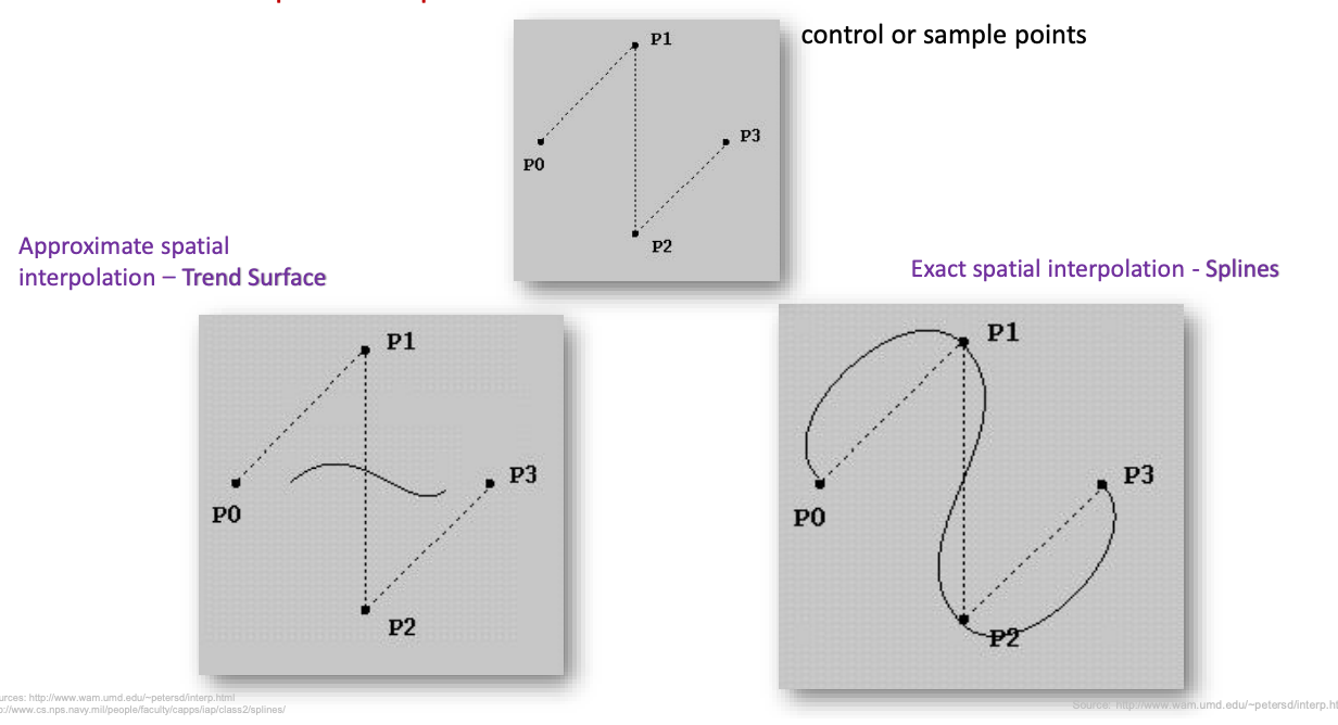
trend surface: fit a general mathematical function (polynomial or regression plane)
resulting curve does not necessarily pass through the sample points - approximates the trend
this is useful when the data has noise or youre more interested in the general pattern than exact values
= approximate interpolation
exact interpolation (spline): creates a curve that passes through all control points
uses a piecewise polynomial function to create a smooth and continuous path through the data
makes it more accurate when exact values matter — (modelling terrain or temp)
= exact interpolation
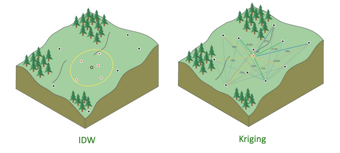
inverse distance weighting (IDW)
weights the points closer to the data source greaterr than those further way - incorporating first law of geog
procedure
superimposes an equally spaced grid of points onto the control/sample points
estimates values at each grid points as a function of their distance from the control/sample points
interpolates between the grid points
IDW estimates values by averaging the values of sample data points in the nieghbourhood (size of window/radius) for each processing point (or raster cell)
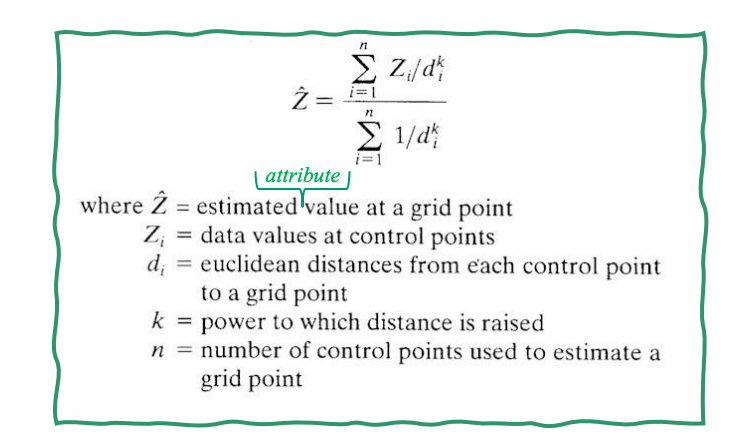
k controls the significance of the surrounding points upon the interpolated values
a higher power results in less influence from distant points and typicallly the generated surface will be smoother
** CALCULATION NEEDED
advantages and disadvantages of the IDW method
most commonly used spatial interpolation method that can applied on large datasets and study areas
the surface resulting from IDW depends on the power exponent k used in the function, and on the size of the window/radius which sample data points are taken for calculation
the size of the window considers certain number of neighbour points, which affects the average values on the estiamted control/sample points and the computational time
the choices of location and the number of control/sample points also have a direct influence on the outcome of the IDW methodx
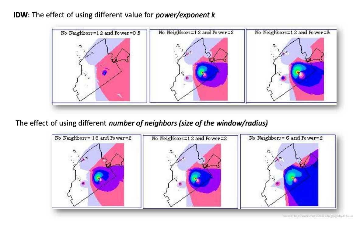
power k controls ho wmuch influence nearby vs distant points have
as power increases, the surfaces becomes sharper and more localized around sample points
Neighbours controls how many sample points are considered for each cell
using fewer neighbours increases detail (but can be noisy), while more neighbours smooth the surface
higher power: tigether, localized influence around points
fewer neighbours: more localized patterns, more variation
kriging interpolation method
the spatial variation of any spatial geogrpahical property is too irregular (heteogen) to be represented by a smooth mathematical function
procedure
kirging superimposes an equally spaced grid of points onto the measured points
interpolates between the grid points giving consideration tos patial autocorrelation (the statistical variation of attribute z values of surrounding points)
estimate the predicted values for each point at location s
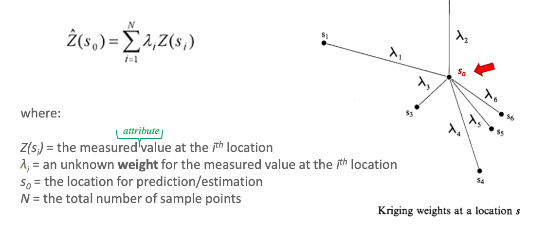
with IDW, the weight only depnds on the dsitance to the prediction location, kriging depends on the overall spatial arrangement (variation), among z values for sample points at distance h (lag interval)
spatial autocorrelation is calculated through the semivariance and semivariogram in order to examine this dependency in spatial variation of attribute values z
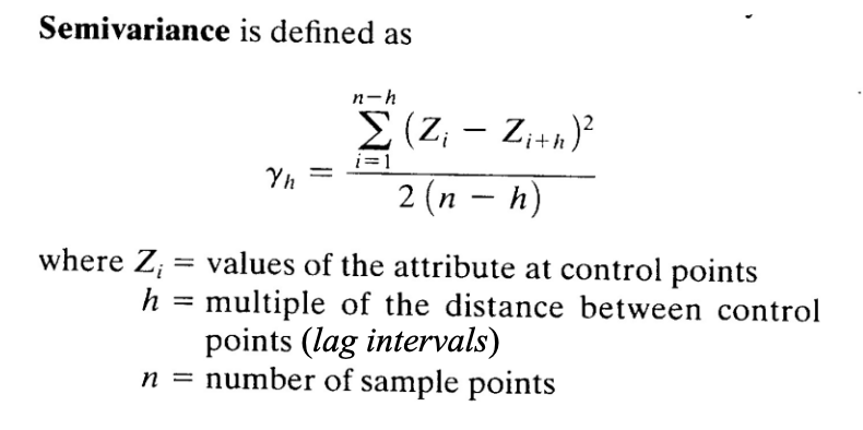
semivariance
half of the variance in the data points over a distance h (lag of intervals) b/w control points
gives an indication of the variations b/w the attribute values of z of sample/control points
the semi variogram is a graph that relates each sample/control point to all other sample/control points with repect to the values of attribute z and distance h (lag intervals) between points
the semivariance and the distance h (lag intervals) are used to construct the semivariogram
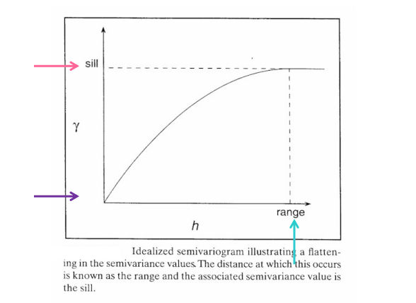
sill: is a particular value of semivariance at which there is no more spatial dependency between the data points
range: gives an indication of distance h (lag intervals) over which spatial dependency occurs
nugget: spatially uncorrelated noise in the data set
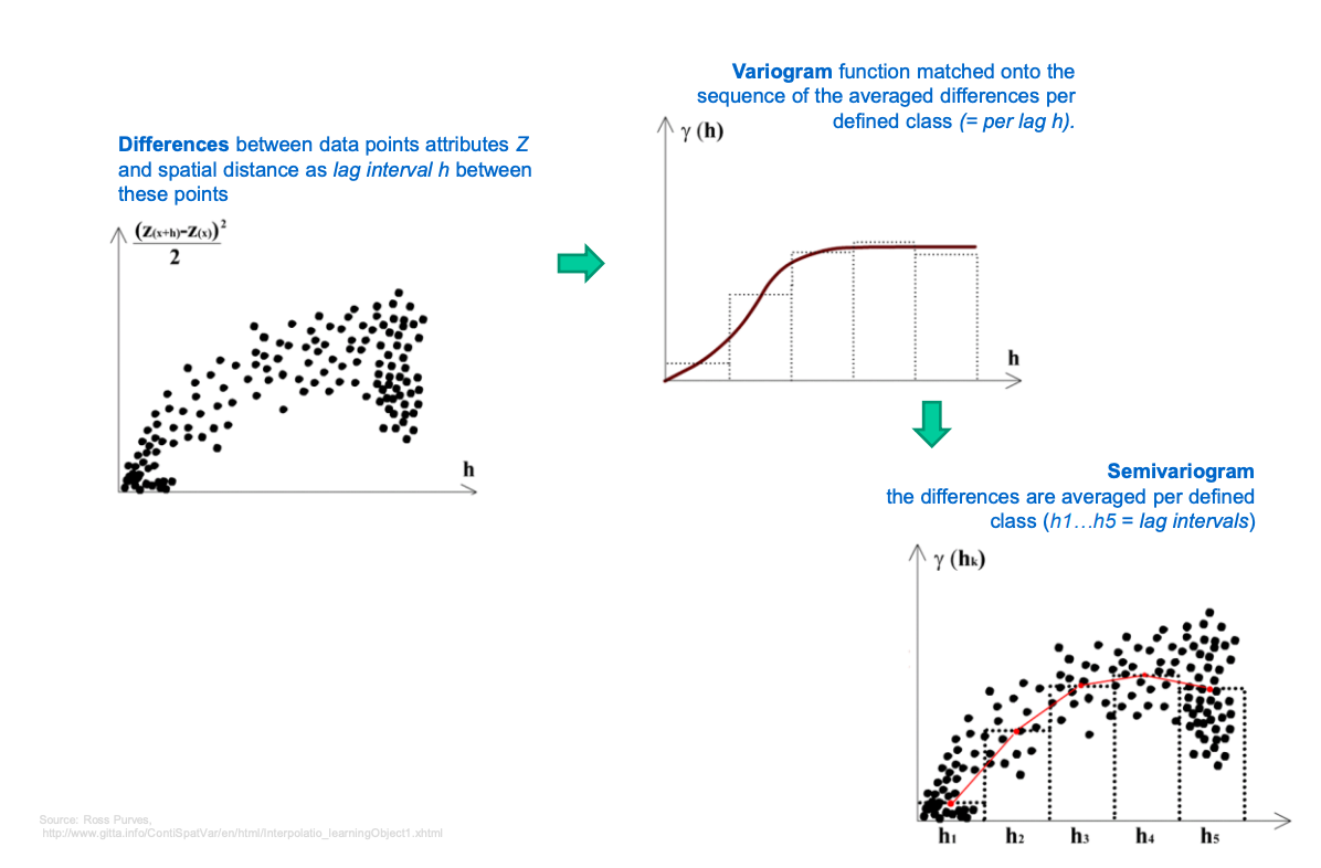
differences: each dot shows the squared difference in value b/w two data points, plotted against teh distancce (lag) h between them
2(Z(x+h)−Z(x))²/2
shows how differences in data values grow as the distance between points increases
data points close together usually have more similar values
variogram: theoretical
raw data grouped into bins
for each lag interval - average semivariance is calculated
averaged values are used to fit a smooth variogram model curve
the curve shows the spatial autocorrelation (how related values are with increasing distance)
semivariogram:
x: lag distance
y: semivariance
each dot = pairwise comparison - red line connects the averaged bins
semivariance increases with distance = points are more different when further apart
where is levels off = range, where distance no longer affects similarity
the semivariogram function increases monotonically with h because the attribute values Z at two near locations most likely are more similar than those at two distant locations
* CALCULATION
advantages and disadvantages of kriging
kirging is an advaned and complex technique that relies heavily on statistical theory and on computing abilities
it is the most useful method when applied on data that contain well defined local trends of the attribute value
the form of semivarigoram is central. to kriging, but it is uncertain if particular functions that estimate semivariogram is a fact the true estimator of the spatial variation in the study area
scale free interpolation technique, can be applied to smaller study areas
typical application of interpolation methods
DTM digital terrain models
can be vector based (TIN) or rraster based (DEM)
measures derived from DTM (DEM and TIN) topographic surfaces
slope: change in elevation over. adefined distance (indicates the incline or steepness of the land surface)
aspect: compass direction in which a slope faces (from north, it is usually expressed clockwise from 0 to 360 degrees)
hillshading or shaded relief: map effect which mimics the sun to highlight hills and valleys (some areas appear to be brighter and some are shadowed)
triangulated irregular networks (TIN) terrain models can provide some of these measures as well as vector isolines (contours)
further research work to advance interpolation methoods
evaluation of interpolation accuracy
methods for comparison of interpolation methods
development of spatio-temporal interpolation methods
development of methods for interpolation of AREAL data
pycnophylactic interpolation: preserve volume in each smallest spatial unit
learning objectives
identify the connections between spatial analysis and spatial modelling
understand the concepts of geodemographics and geosimulation
apply spatial analysis and spatial modelling approaches to real problems
lecture 12
geodemographics
main focus
profiling people based on the location where they live
understanding the composition of human settlements in different kind of neighbourhoods
creation of market segmentation systems
neighbourhood classification systems: segmentation systems - since the mid 1930s
the widespread commericial applications only began in the late 70s and early 80s with the launch of the PRIZM system
geodemographics require
various spatial data analysis methods
census and postal geography data
large geospatial and socio-economic datasets
GIS software for analysis, mapping and display
michael j weiss
1988: clustering of america
1994 latitudes and attitudes
2000: the clustered world: how we live, what we buy, and what it all means about who we are
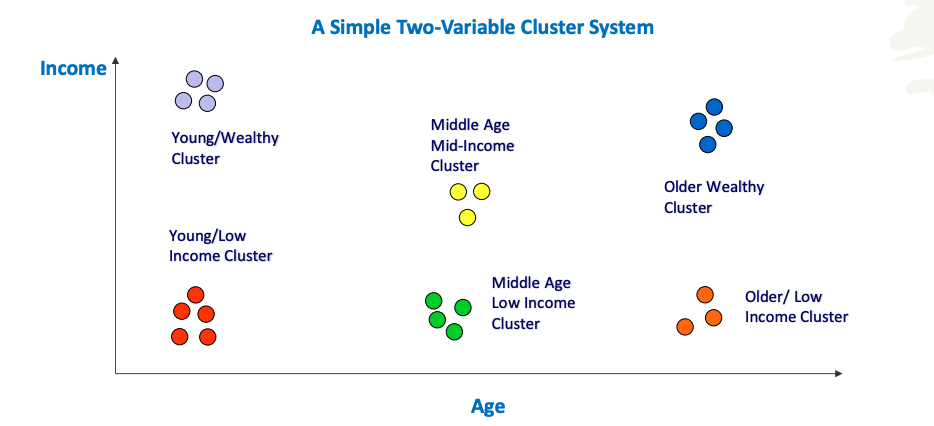
the goal of segmentation system is classifying neighbourhoods into homogeneous types of clusters
find groups or clusters of neighbourhoods that are similar to eachother, demographically and in terms of lifestyle
questions that segmentation systems can answer
who are my best customers
what are the social values and spending habits. ofmy customers
where can i find most of my customers
where should i target to meet my specified audiences
where are my fundraisers
where are the communities for high priority locations to set up fly shot clilcs?
what are the consumers traffic patterns and traffic volume
PRIZM
environics
68 segments
spatial data analysis
spatial analysis of networks
case studies related to the
occurence of traffic accidents on highways
locatioon of stores alongside roads
incidence of crime on streets or
contamination along rivers
space time analysis
study of things change across both space and time simultaneously
combines geography with temporal pattens to help us understand complex processes that unfold dynamically
ex: covid 19 - spatial element: cities/countries affected, temporal elemts: weekly case data
geosimulations
suggestions for the second law of geog
spatial heterogeneity or nonstationary implies that geographic variables exhibit uncontrolled variance
there is no concept of an average place on the earths surface comparable to an average human
reaction
complex adaptive systems theory suggest that near can be sufficient
simple and local interactions among entities of the system at local level can produce complex behaviour and patterns at global level, that are not completely predictable or controllable
in the real world - everything is process
space and time need to be considered together = spatio-temporal analysis and modelling
complex system theory can deal with processses that operate in space and time
geocomputation and geosimulation are new fields of GIScience that are based on complex system theory, adn they contribute to advancememnt of spatial analysis and modelling of complex dynamic spatial systems
ex: john conweys game of life/urban growth geosimulations
sagregation model - people tend to live in nieghbourhoods where 50% or mrore are like themselves
cellular automata - geosimulation models: modeling regional urbanization process
complex systems theory permits modelling od wide range of spatial and geographical dynamic phenomena especially when integrated with GIS and geospatial data
human behaviour as a complex dynamic spatial system
agent based modelling approach can be used to represent spatio-temporal dynamics of human evacuation behaviour