AP_Microeconomics Unit 5 Notes
5.1 Changes in Factor Demand and Supply
5.1.1 Demand for Labor Shifters
Price of Output: Higher prices for products lead to an increase in demand for labor, as employers seek to capitalize on higher potential profits.
Derived Demand: The demand for a factor of production or input that is dependent on the demand for the final goods or services produced with that resource.
Worker Productivity: More productive workers increase demand for labor because they contribute more effectively to production.
Prices of Other Resources: The costs of substitute and complementary goods influence labor demand. For example, if machinery becomes cheaper, firms may opt to purchase machinery over hiring more labor.
5.1.2 Labor Demand Scenarios
When there’s an increase in demand for microprocessors, this leads to a corresponding increase in demand for assemblers to produce them.
A price increase for plastic piping parallels an increase in demand for copper piping, affecting labor related to these materials.
A rise in demand for small homes can lead to a decrease in demand for lumber, impacting jobs in lumber production.
Conversely, a decrease in the price of trains results in a decrease in demand for trucks in logistics.
A decrease in price of sugar can lead to an increase in demand for aluminum for soda producers as manufacturers adjust their costs.
Increased education/training correlates with an increase in demand for skilled labor, as employers seek out highly trained individuals.
5.1.3 Supply of Labor Shifters
Education and Training: Greater education and specialized skills can increase the labor supply as more individuals qualify for employment.
Availability of Alternatives: The presence of job options can influence people’s willingness to enter the labor market.
Immigration/Mobility: Movement across regions or countries serves to augment or reduce local labor supply depending on the quantity of incoming workers.
Cultural Expectations: These norms can influence the demographics of labor available in certain fields.
Distribution by Age: Different age groups have varying levels of participation in the workforce, affecting overall labor supply.
Leisure Preferences: If individuals prefer leisure over work, it limits the labor supply available to employers.
5.1.4 Competitive Labor Market Characteristics
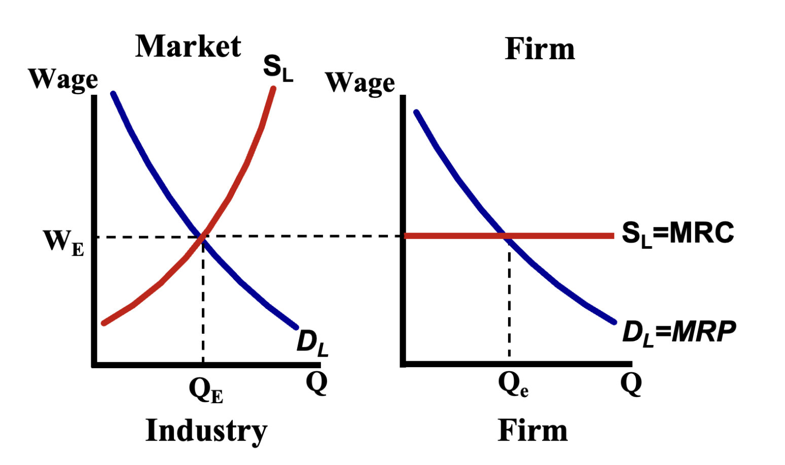
Features of a competitive labor market include numerous firms and employees, leading to conditions where no single firm can exert control over wage rates. Firms are considered wage takers, accepting the prevailing market wage without influence on it.
5.2 Profit-Maximizing Behavior
MRP Calculation: The Marginal Revenue Product (MRP) is calculated as MRP = MP (Marginal Product) x MR (Marginal Revenue). Firms will hire labor up until the point where MRP equals Marginal Resource Cost (MRC), optimizing their profit potential.
5.2.1 Perfect Competition Characteristics
Multiple firms compete for labor, enabling workers to make choices based on wage offers.
No single firm can influence wage rates, as they are considered wage takers.
The market achieves equilibrium where the marginal revenue product intersects with the labor supply curve, maximally utilizing labor resources.
5.2.2 Monopsony Characteristics
In a monopsony, a single firm dominates the labor market, leading to wages that must increase to attract additional labor. The Marginal Factor Cost (MFC) typically exceeds the supply curve.
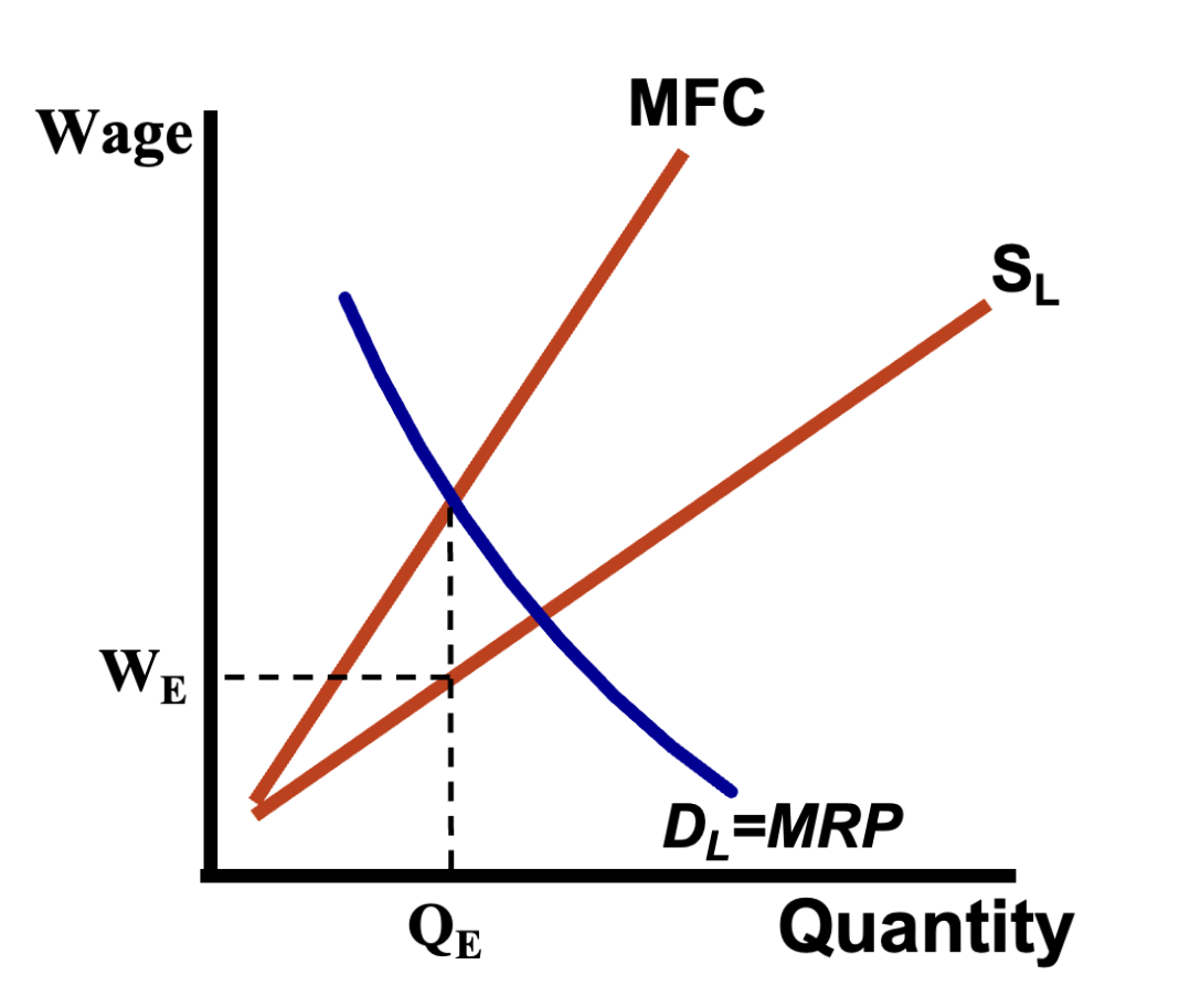
5.2.2 Monopsony vs. Perfect Competition
Comparatively, a monopsonist hires fewer workers at lower wages than in a perfectly competitive market, affecting overall employment levels and wage standards.
The marginal revenue product of labor intersects with the supply curve to define optimal labor quantities under these conditions.
5.2.3 Job Jungle Overview
Employees typically start in low-skilled roles but can advance to high-skilled positions through education and training. Wage negotiations occur based on the concept of marginal productivity. Variances in worker assistance depend on skill levels and job statuses.
5.3 Important Formulas and Concepts
MRP = MP x MR: Used for calculating the marginal revenue product of labor.
MRC: Marginal Resource Cost; the additional cost incurred by employing one extra unit of a resource.
Equilibrium Wage: The wage level at which supply meets demand in a competitive labor market.
Monopsony Wage: The wage set by a monopsonist, typically lower than in a competitive market.
Least Cost Rule:
To minimize production costs, the ratio of the marginal product of each input (labor and capital) should be equal to the ratio of their respective prices, ensuring efficient resource allocation.