AP Calculus BC Unit 7: Differential Equations (Slope Fields, Euler’s Method, Separable IVPs, Exponential and Logistic Models)
Understanding Differential Equations and Their Solutions
A differential equation is an equation that relates an unknown function (often written as
y
to one or more of its derivatives (like
y'
). In regular algebra, you usually solve for a number. In differential equations, you are solving for a function—a whole rule that describes how a quantity changes.
Differential equations connect naturally to earlier calculus ideas like related rates: in related rates, we modeled how one changing quantity is related to another using derivatives. Differential equations do something similar, except the “unknown” is the entire function whose rate of change is described.
The big idea is this: many real processes are easiest to describe by how they change moment-to-moment rather than by a direct formula. For example, “population increases at a rate proportional to the population” is naturally written in terms of a derivative.
Key vocabulary: order, solutions, and initial conditions
The order of a differential equation is the highest derivative that appears. For example,
y' = x^2
is first-order, while
y'' + y = 0
is second-order (not a major focus in this unit’s solving techniques).
A solution to a differential equation is a function that makes the equation true wherever it is defined. If you propose a function, you can verify it by substituting it into the differential equation and checking that both sides match.
A general solution is a family of solutions containing an arbitrary constant (often
C
). Many first-order differential equations have infinitely many solutions because you can shift the solution curve up or down.
An initial value problem (IVP) is a differential equation plus an initial condition like
y(x_0)=y_0
. The initial condition picks out one specific member of the family (a particular solution).
Why this matters: on the AP exam, a huge fraction of differential equation work is about interpreting what a differential equation is saying, approximating its solutions, and solving separable equations with an initial condition.
Notation you must recognize (they all mean “derivative”)
In AP Calculus BC, the same derivative may appear in different forms. You need to be fluent in switching between them.
| Meaning | Common notations |
|---|---|
| derivative of %%LATEX6%% with respect to %%LATEX7%% | %%LATEX8%%, %%LATEX9%% |
| differential equation written “separated” | %%LATEX10%% or %%LATEX11%% |
A common misconception is to treat
\frac{dy}{dx}
as a simple fraction all the time. In general, it represents a derivative. But in separable differential equations, rewriting in “fraction-like” form is a powerful, valid technique.
What it means to solve (or not solve) a differential equation
There are three main outcomes you’ll see in this unit:
- Solve exactly (usually via separation of variables): you find a formula for
y
(sometimes implicit).
- Describe qualitatively: you sketch behavior from a slope field without an explicit formula.
- Approximate numerically (Euler’s method): you compute approximate values of
y
at specified
x
-values.
Even when an exact solution exists, AP problems may still ask for numerical approximations or qualitative interpretations—because those skills mirror real applied work.
When “solving” is just antidifferentiating
If the differential equation gives the derivative of a function equal to a function of the independent variable alone, you can solve by integrating both sides. For example, if
\frac{dy}{dx}=x^2
then solving means finding an antiderivative:
y=\int x^2\,dx
which produces
y=\frac{x^3}{3}+C
This idea is part of the bigger theme: differential equation problems often involve “undoing a derivative.”
Exam Focus
- Typical question patterns:
- “Verify that a given function is a solution to the differential equation, then use an initial condition to find the constant.”
- “Given
\frac{dy}{dx}
determine whether a function is increasing/decreasing or concave up/down at a point.”
- “Interpret what the differential equation says about a real-world situation (units and meaning of terms).”
- Common mistakes:
- Forgetting that solutions are functions (not single numbers), so you must include a constant in general solutions.
- Plugging into the differential equation incorrectly (especially mixing up
y
and
y'
).
- Treating an initial condition like
y(0)=5
as if it changes the differential equation itself—it only selects one solution.
Slope Fields and Qualitative Solution Behavior
A slope field (also called a direction field) is a picture that tells you the slope of solution curves at many points in the plane. Since a first-order differential equation gives
y'
as a function of
x
and
y
, it tells you the slope at every point
(x,y)
. A slope field visualizes that information.
Why this matters: many differential equations cannot be solved with elementary formulas, but you can still understand their behavior—where solutions rise, fall, level off, or approach equilibrium.
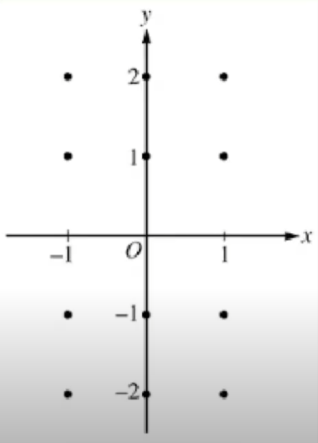
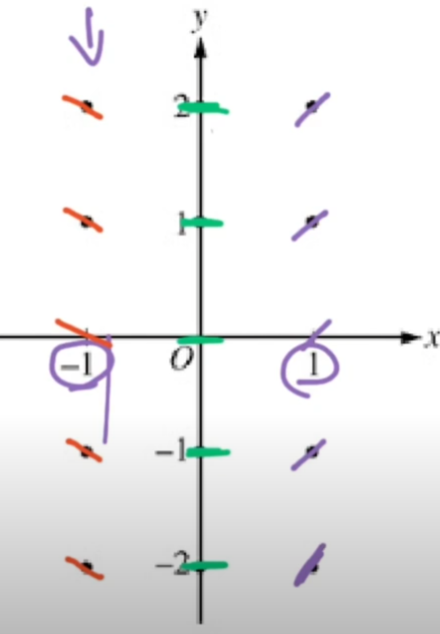
How to construct a slope field (mechanics)
To construct a slope field, you plug the point’s coordinates into the differential equation to get the slope at that point, then draw a small line segment with that slope. In other words: evaluate the right-hand side at the point and draw that as the slope.
For example, for the equation
\frac{dy}{dx}=x
the slope depends only on
x
. So at
x=-1
the slope is
-1
no matter what
y
is.
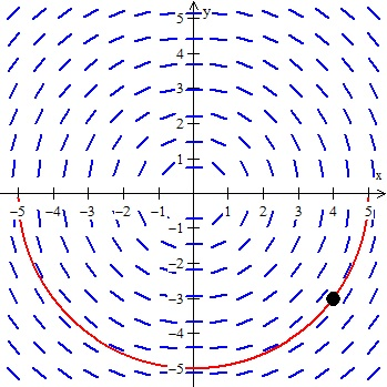
How to read a slope field
If you have a differential equation
\frac{dy}{dx}=F(x,y)
then at each point
(x,y)
the slope of the solution curve is
F(x,y)
.
To sketch solution curves:
- Pick a starting point (often an initial condition).
- Follow the little line segments, drawing a smooth curve that is always tangent to the segment directions.
When the AP exam asks for a solution curve from a slope field, the core skill is to “flow” with the slopes. Because this is by hand, it doesn’t have to be exact, but it should consistently track the tangent directions.
Two important clarifications:
- Solution curves cannot cross (in typical AP settings where
F(x,y)
is well-behaved). If they crossed, you would have two different slopes at the same point, which contradicts the idea that the differential equation assigns a unique slope.
- A slope field gives local information (slope at a point), not a direct formula for the entire curve.
Isoclines: places where the slope is constant
An isocline is a curve where the slope
\frac{dy}{dx}
has a constant value
k
:
F(x,y)=k
On a slope field, isoclines help you organize the picture: along that curve, all the direction segments have the same slope. You won’t always be asked to find isoclines, but the idea helps you reason about patterns.
Equilibrium solutions (constant solutions)
An equilibrium solution is a constant solution
y=c
such that the derivative is zero everywhere along that horizontal line. For equations of the form
\frac{dy}{dx}=G(y)
equilibria occur when
G(c)=0
These matter especially for autonomous differential equations (where the right side depends only on
y
). Equilibrium solutions often represent steady states like a stabilized population.
Stability intuition (qualitative)
If nearby solutions move toward an equilibrium as
x
increases, it’s stable. If nearby solutions move away, it’s unstable. You can often decide this by checking the sign of
G(y)
above and below the equilibrium.
Worked example: sketching behavior from a differential equation
Suppose
\frac{dy}{dx}=y(1-y)
This is an autonomous equation. Look for equilibria:
y(1-y)=0
So equilibria are
y=0
and
y=1
Now analyze the sign of
y(1-y)
:
- If
0