11 - The Influence of Fiscal and Monetary Policy on Aggregate Demand

The Influence of Fiscal and Monetary Policy on Aggregate Demand

This note covers the influence of fiscal and monetary policy on aggregate demand (AD), including the interest-rate effect, how the central bank (CB) uses monetary policy to shift the AD curve, the two ways fiscal policy affects aggregate demand, and arguments for and against using policy to stabilize the economy.

Earlier Chapters

• Discussed the long-run effects of fiscal policy on interest rates, investment, and economic growth.

• Addressed the long-run effects of monetary policy on the price level and inflation rate.

• This chapter focuses on the short-run effects of fiscal and monetary policy, which operate through aggregate demand.

Aggregate Demand Curve

• The AD curve slopes downward due to:

  • The wealth effect (P - C)

  • The interest-rate effect ← the most important (P - I)

  • The exchange-rate effect (P - NX)

• We will use a supply-demand model for the money market to explain the interest-rate effect and how monetary policy affects aggregate demand.

Monetary Policy and AD

1. Money Market - Theory of Liquidity Preference

• Keynes’ theory of liquidity preference explains the factors determining the economy’s interest rate.

• According to the theory, the interest rate adjusts to balance the supply and demand for money (short-term → sticky)

• If the expected rate of inflation is constant, the real and nominal interest rate move in the same direction.

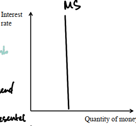
Money Supply

• Money supply i controlled by central bank

• The quantity of money supplied does not depend on interest rate

• The fixed MS is represented by a vertical curve

  

Money Demand

• Money demand reflects how much wealth people want to hold in liquid form (tổng tài sản có tính lỏng cao)

• Household wealth includes:

  • Money: liquid but pays no interest.

  • Bonds: pay interest but are not as liquid.

• A household’s money demand reflects its preference for liquidity.

• The opportunity cost of holding money is the interest that could be earned on interest-earning assets.

• Variables influencing money demand: income (Y), interest rate (r), and price level (P).

  • Y rises → C rises → MD rises

  • P rises → MD (nominal) rises (need more money for transactions)

  • Interest rate rises → S rises → C falls → MD falls

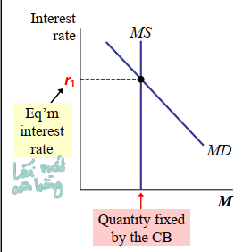
Equilibrium in the Money Market

• The money supply (MS) curve is vertical because changes in the interest rate do not affect MS, which is fixed by the central bank (CB).

• The money demand (MD) curve is downward sloping; a fall in the interest rate increases money demand.

• Equilibrium interest rate: the rate at which the quantity of money demanded equals the quantity of money supplied.

  

2. How the Interest-Rate Effect Works

• A fall in P reduces money demand, which lowers r

  

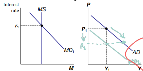
  • P falls → MD falls → MD curve shifts down

  • A fall in r increases I and the quantity of g&s demanded

• Monetary policy is how the monetary authority controls the money supply, often targeting an interest rate to promote growth and stability.

• The central bank's policy instrument is the money supply (MS), which it uses to change the interest rate and shift the AD curve.

• Expansionary monetary policy increases the money supply, lower interest rate => shifts AD right

• Contractionary monetary policy decreases the money supply, higher interest rate => shifts AD left

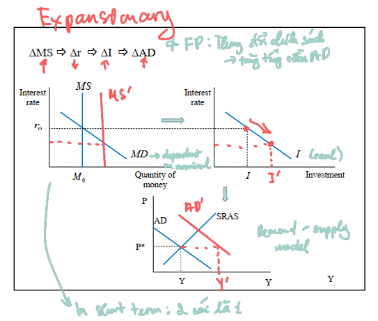
3. Effect of Changes in Money Supply

• An increase in MS lowers the interest rate, encourages investment, and increases the quantity of goods and services demanded at any given price level, shifting AD to the right.

  • \Delta MS \rightarrow \Delta r \rightarrow \Delta I \rightarrow \Delta AD

  • MS rises → shifts right → new equilibrium: r drops

  • Interest rates decreases → Investment (and some C) increases

  • I directly raises AD → AD shifts right

  • When the Fed increases money supply, the equilibrium interest falls, which increases the quantity of g&s demanded at a price level (giải thích cho graph 3 vì sao gióng ngang từ P sang =>increased quantity demanded at the same price level)

    

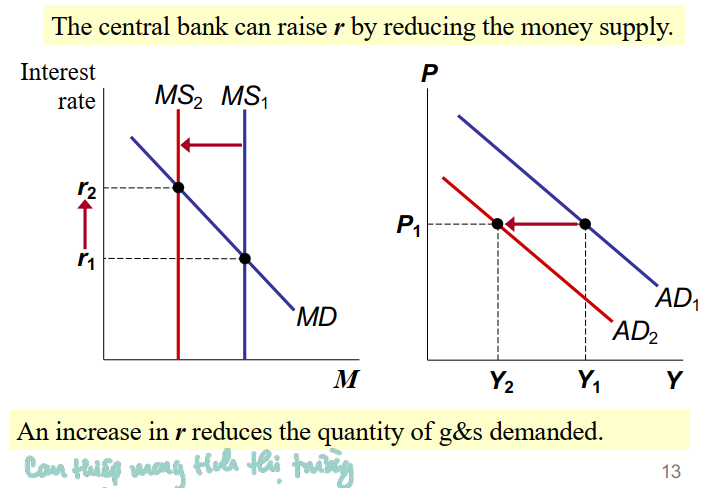
• A decrease in MS raises the interest rate, discourages investment, and reduces the quantity of goods and services demanded at any given price level, shifting AD to the left.

• The central bank can raise the interest rate by reducing the money supply. An increase in the interest rate reduces the quantity of goods and services demanded.

  

• Note: Monetary policy can be described either in terms of the money supply or in terms of interest rates

  → Changes in monetary policy an be viewed either in terms of a changing target for the interest rate or in terms of a change in the money supply

Fiscal Policy and AD

• Fiscal policy involves setting the level of government spending and taxation by government policymakers.

• Expansionary fiscal policy involves an increase in government purchases (G) and/or a decrease in taxes (T), shifting AD to the right.

• Contractionary fiscal policy involves a decrease in government purchases (G) and/or an increase in taxes (T), shifting AD to the left.

1. The Multiplier Effect

• The multiplier effect refers to the additional shifts in AD that result when fiscal policy increases income and thereby increases consumer spending.

• If the government buys \$20 billion of planes from Boeing, Boeing’s revenue increases by \$20 billion. This is distributed to Boeing’s workers (as wages) and owners (as profits or stock dividends).

• These people are also consumers and will spend a portion of the extra income, causing further increases in aggregate demand.

  

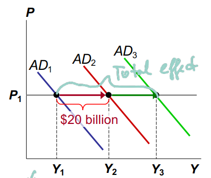
• A \$20 billion increase in G initially shifts AD to the right by \$20 billion. The increase in Y causes C to rise, which shifts AD further to the right.

Marginal Propensity to Consume (MPC)

• The size of the multiplier effect depends on how much consumers respond to increases in income.

• Marginal propensity to consume (MPC) is the fraction of extra income that households consume rather than save (MPC = \Delta C / \Delta Y_d).

• For example, if MPC = 0.8 and income rises \$20 billion, consumption (C) rises \$16 billion and saving (S) rises \$4 billion.

• Bất kể là thành phần bào thay đổi thì dều tăng/giảm gấp nhiều lần so với lượng ban đầu

Formula for the Multiplier

• Notation:

  • \Delta G is the change in government purchases.

  • \Delta Y is the ultimate change in income.

  • \Delta C is the ultimate change in consumption.

• Y = C + I + G + NX (identity)

• \Delta Y = \Delta C + \Delta G (I and NX do not change)

• \Delta Y = MPC \cdot \Delta Y + \Delta G (because \Delta C = MPC \cdot \Delta Y)

• Solving for \Delta Y:

  • \Delta Y = \frac{1}{1 - MPC} \cdot \Delta G

• The spending multiplier is \frac{1}{1 - MPC}.

• A bigger MPC means changes in Y cause bigger changes in C, which cause more changes in Y.

• Examples:

  • If MPC = 0.5, the multiplier = 2.

  • If MPC = 0.75, the multiplier = 4.

  • If MPC = 0.9, the multiplier = 10.

Changes in Taxes

• A tax cut increases households’ take-home pay.

• Households respond by spending a portion of this extra income, shifting AD to the right.

• The size of the shift is affected by the multiplier and crowding-out effects.

• Another factor is whether households perceive the tax cut to be temporary or permanent; a permanent tax cut causes a bigger increase in C than a temporary tax cut.

• Công cụ thuế yếu hơn công ụ chi tiêu chính phủ (T<G) do một phần thuế đc giảm sẽ đưa vào savings thay vì sử dụng hoàn toàn cho chi tiêu

The Multiplier and Taxes

• Notation:

  • \Delta T is the change in taxes.

  • \Delta Y is the ultimate change in income.

  • \Delta C is the ultimate change in consumption.

• Y = C + I + G + NX (identity)

• \Delta Y = \Delta C (I and NX do not change)

• \Delta Y = MPC \cdot (\Delta Y - \Delta T) (because C is a function of Y-T)

• Solving for \Delta Y:

  • \Delta Y = \frac{1}{1 - MPC} \cdot (-MPC \cdot \Delta T)

• The tax multiplier is \frac{-MPC}{1 - MPC}.

Other Applications of the Multiplier Effect

• Each \$1 increase in G can generate more than a \$1 increase in aggregate demand.

• This is also true for the other components of GDP.

• Example: Suppose a recession overseas reduces demand for U.S. net exports by \$10 billion. Initially, aggregate demand falls by \$10 billion. The fall in Y causes C to fall, which further reduces aggregate demand and income. If MPC is 0.8 then total change = -10 × 1/(1-0.8) = 50 bil

2. The Crowding-Out Effect

• Fiscal policy also affects AD in the opposite direction.

• A fiscal expansion raises the interest rate (r), which reduces investment, which reduces the net increase in aggregate demand.

• The size of the AD shift may be smaller than the initial fiscal expansion.

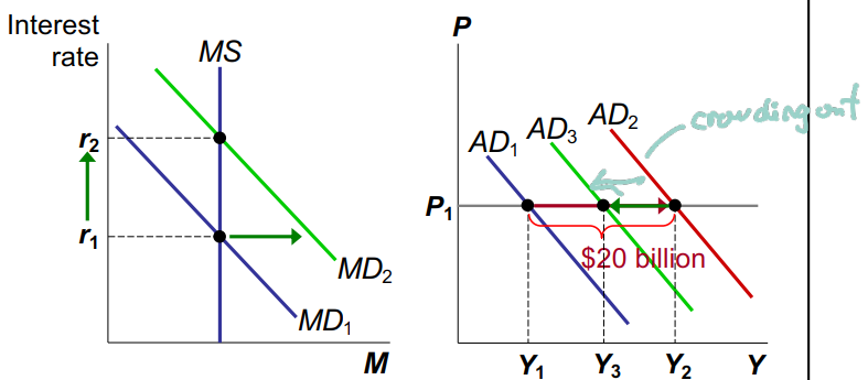
• This is called the crowding-out effect: the offset in aggregate demand that results when expansionary fiscal policy raises the interest rate and thereby reduces investment spending.

• A \$20 billion increase in G initially shifts AD to the right by \$20 billion, but higher Y increases MD and r (MS is fixed), which reduces AD from I decreasing.

  

Using Policy to Stabilize the Economy

• Economic stabilization has been a goal of economic policy.

• Economists debate how active a role the government should take to stabilize the economy.

• Active stabilization policy involves using policies to smooth the fluctuation of demand and output.

• Fiscal policy (increase in G or/and reduce T) if the economy is in a recession (GDP falls below its natural rate) and vice versa.

1. The Case for Active Stabilization Policy

• Keynes: “Animal spirits” cause waves of pessimism and optimism among households and firms, leading to shifts in aggregate demand and fluctuations in output and employment.

• Also, other factors cause fluctuations, e.g., booms and recessions abroad and stock market booms and crashes.

• If policymakers do nothing, these fluctuations are destabilizing to businesses, workers, and consumers.

• Proponents of active stabilization policy believe the government should use policy to reduce these fluctuations.

  • When GDP falls below its natural rate, use expansionary monetary or fiscal policy to prevent or reduce a recession.

  • When GDP rises above its natural rate, use contractionary policy to prevent or reduce an inflationary boom.

2. The Case Against Active Stabilization Policy

• Policies also work with a long lag.

  • Inside lag: the time between a shock and policy action (recognition lag, decision lag, and implementation lag).

  • Outside lag: the time between policy action and its influence on the economy (impact lag).

• Fiscal policy works with a long lag because changes in G and T require the agreement of Congress, and the legislative process can take months or years.

• Monetary policy also affects the economy with a long lag because firms make investment plans in advance, so I takes time to respond to changes in r. Most economists believe it takes at least 6 months for monetary policy to affect output and employment.

• Critics of active policy argue that such policies may destabilize the economy rather than help it because by the time the policies affect aggregate demand, the economy’s condition may have changed.

• These critics contend that policymakers should focus on long-run goals like economic growth and low inflation.

Automatic Stabilizers

• Automatic stabilizers are tax structures and government spending programs that stimulate or depress aggregate demand when necessary without any deliberate policy change from policymakers.

• Examples:

  • System of income taxes: automatically reduces taxes when the economy goes into a recession (Y decrease => T decrease).

  • Unemployment insurance benefits, welfare benefits, or other forms of income support: In recession, more people apply for public assistance (welfare, unemployment insurance).

• Without these automatic stabilizers, output and employment would probably be more volatile than they are.

Conclusion

• Policymakers need to consider all the effects of their actions.

• When the government cuts taxes, it should consider the short-run effects on aggregate demand and employment and the long-run effects on saving and growth.

• When the CB reduces the rate of money growth, it must take into account not only the long-run effects on inflation but the short-run effects on output and employment.