Simple/Filtered Back Projection, Radon Transform

Summary

Each of the following are different methods to constructing a CT image:

Simple Back Projection - in lectures and video (but not in textbook)

Filtered Back Projection - in lectures, textbook and video

Radon Transform - in lectures and textbook

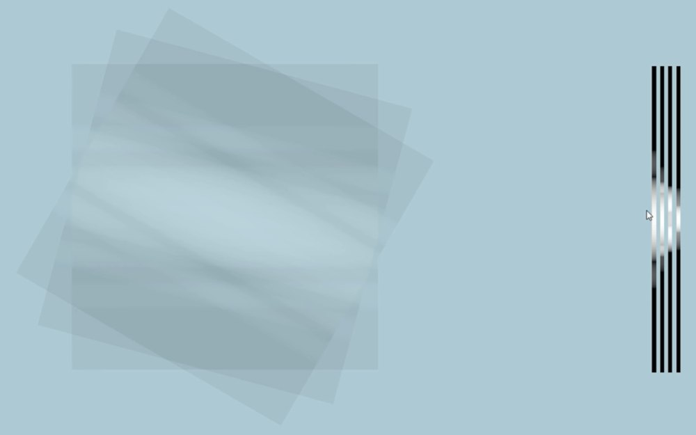
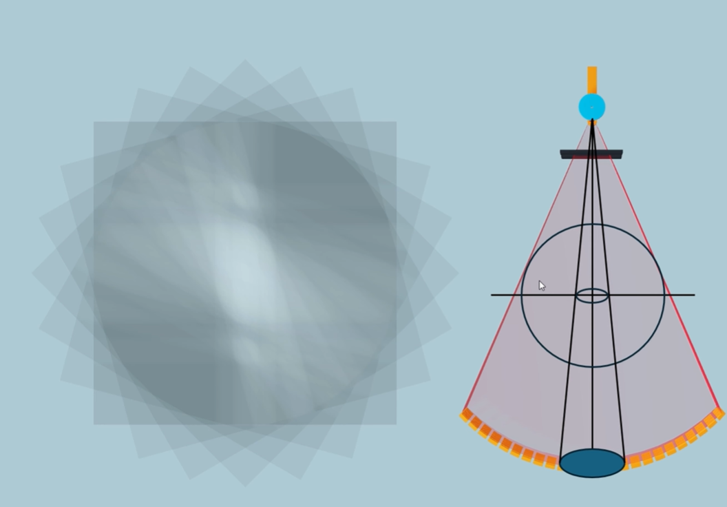
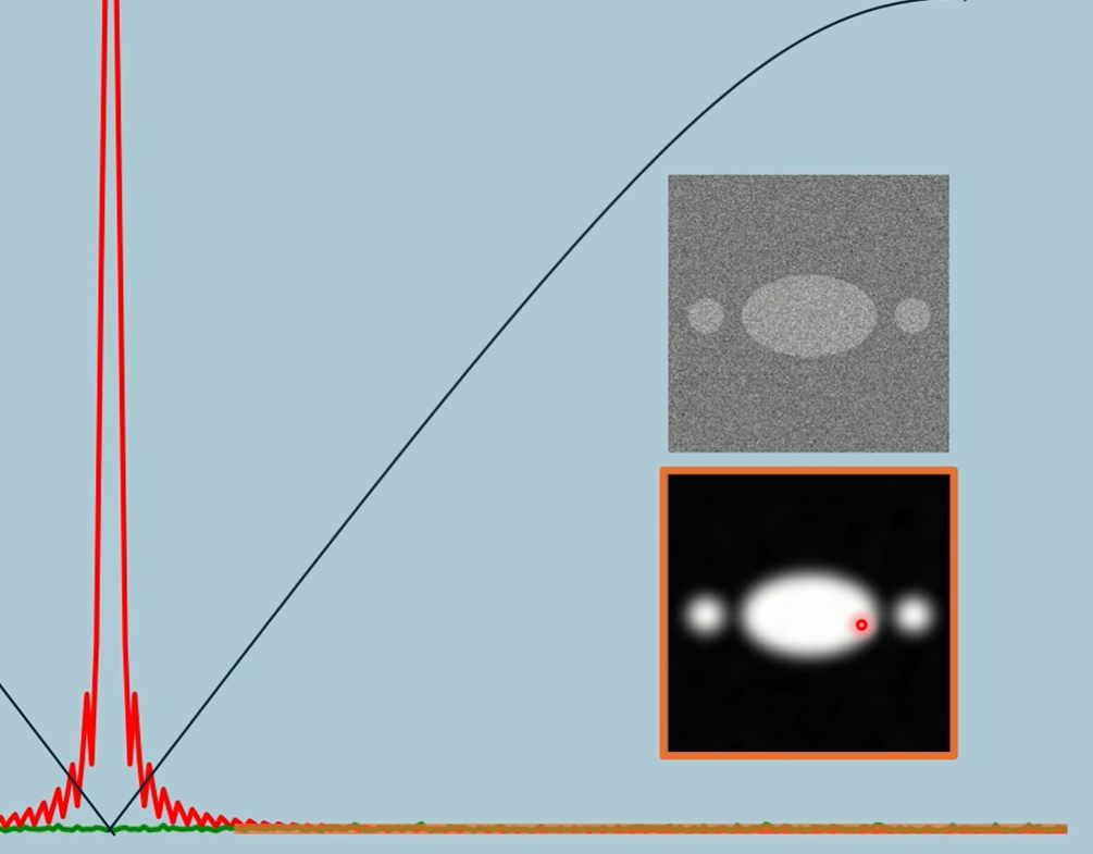
Simple Back Projection: Taking a projection, stretch it back, and then layering with multiple projections. Suffers from blurring.

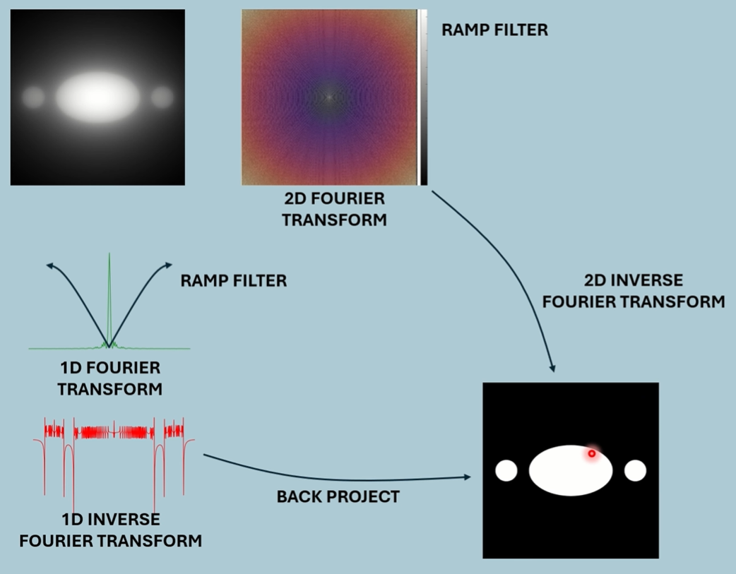
Radon Transform: Method to collect attenuation data. 1D Fourier Transform a projection, use that to build up a 2D Fourier Transform. Can either filter the 2D Fourier image and inverse transform, or can use each 1D Fourier Transform for filtered back projection.

Filtered Back Projection: Uses Radon Transform to gather frequency data for projections, filters them, then back projects.

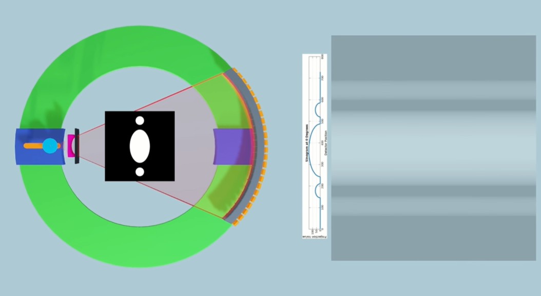
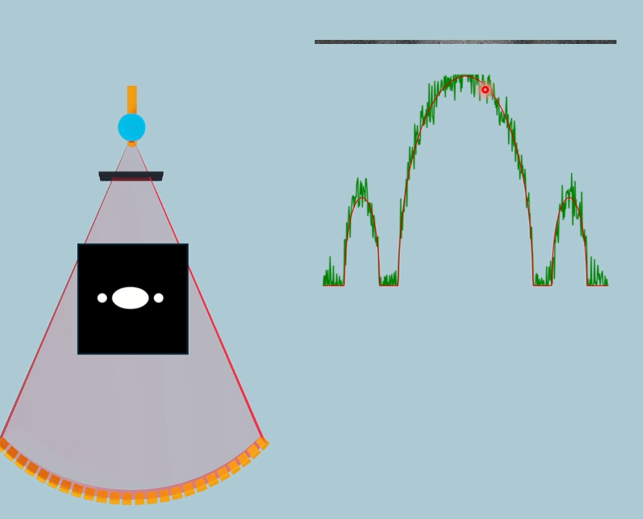
Video + Lectures - Simple Back Projection

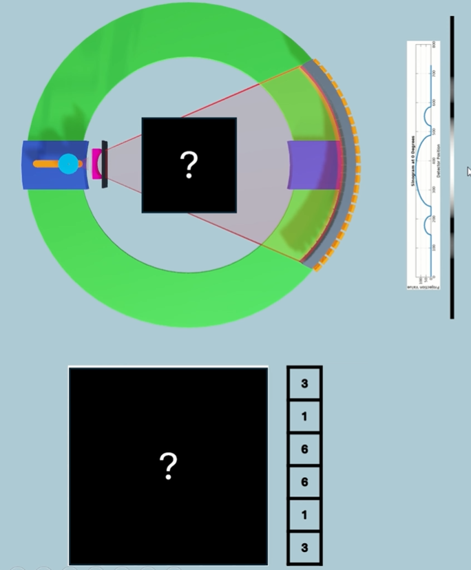
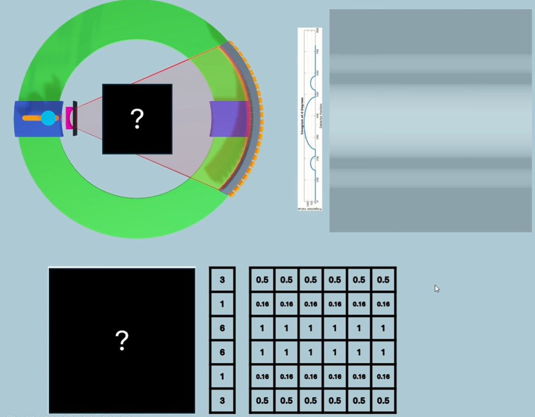
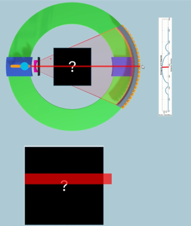
How we can take the initial data that we've generated from all the projections around the patient and figure out what the attenuation value is for different spatial locations within our patient.

Sinogram is raw data. Needs to be cleaned up.

Then we need to find the attenuation value for each voxel within a specific slice.

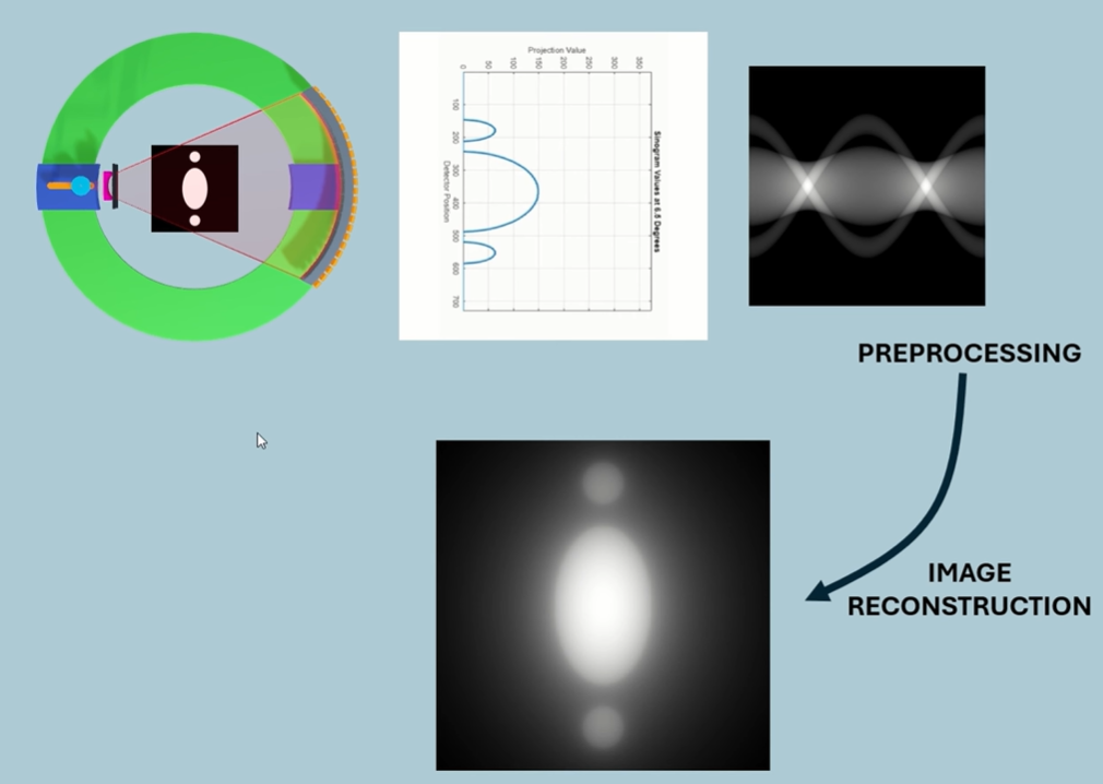
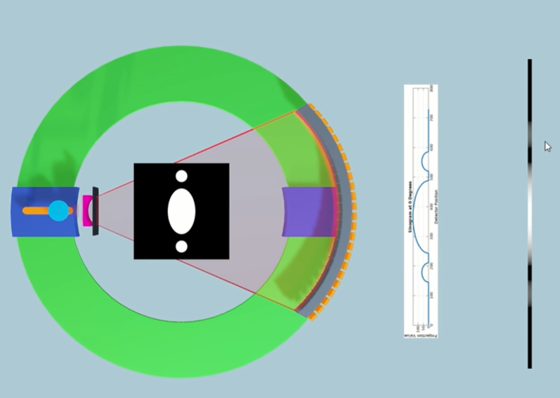
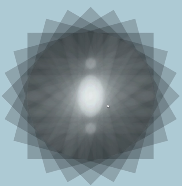
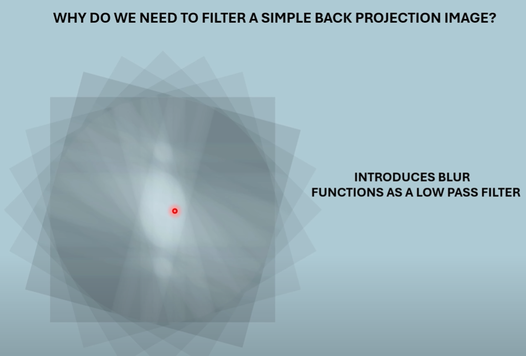
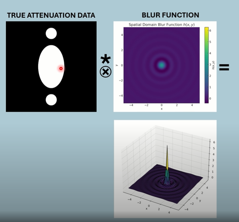
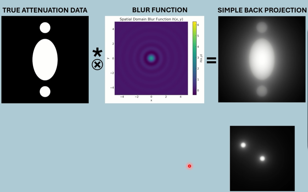
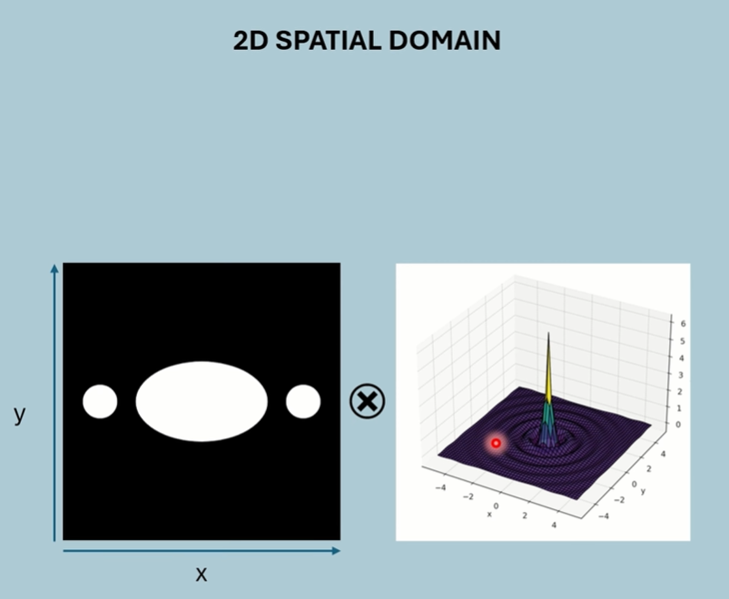
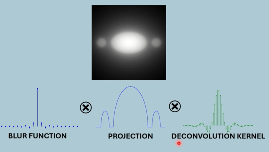
Now we need a process to take this simple back projection data, which has this inherent blur in the image because of that smearing out of data, and we need a way of taking out that blur, of deblurring the image. And it turns out there's a mathematical process for how that blur has been introduced into the image, and that's what's known as convolution. It's taken the true data that's come through our projections, and it's convoluted with a blur function because of our rotation around the patient and the smearing of the data.

It turns out that we can deconvolute the image through a deconvolution kernel or filter, and it will take this data and it will convert it into data that looks like this, a much crisper dataset.

Equations

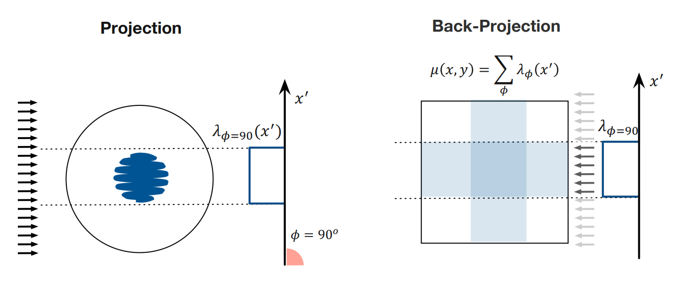
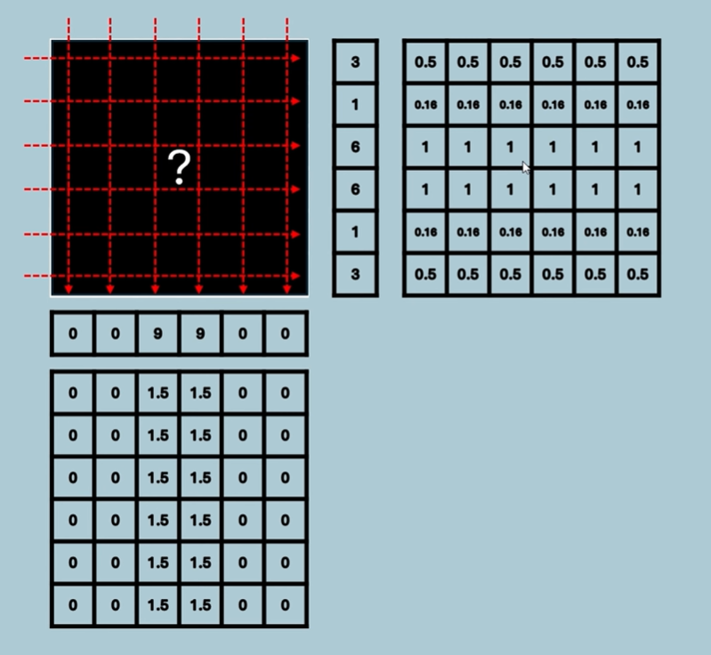
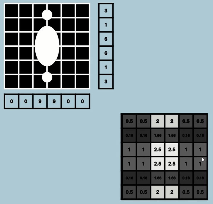
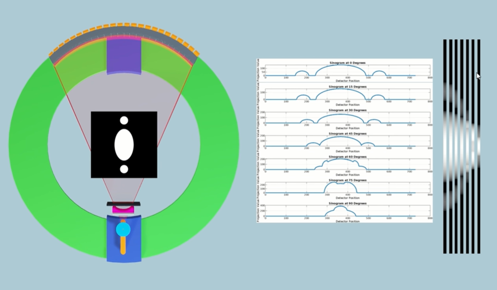
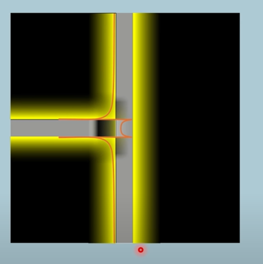
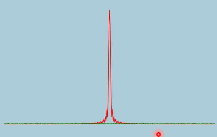
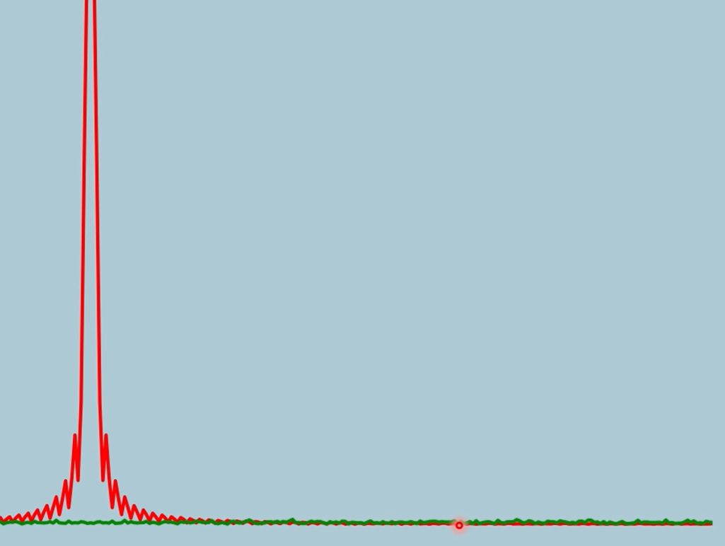
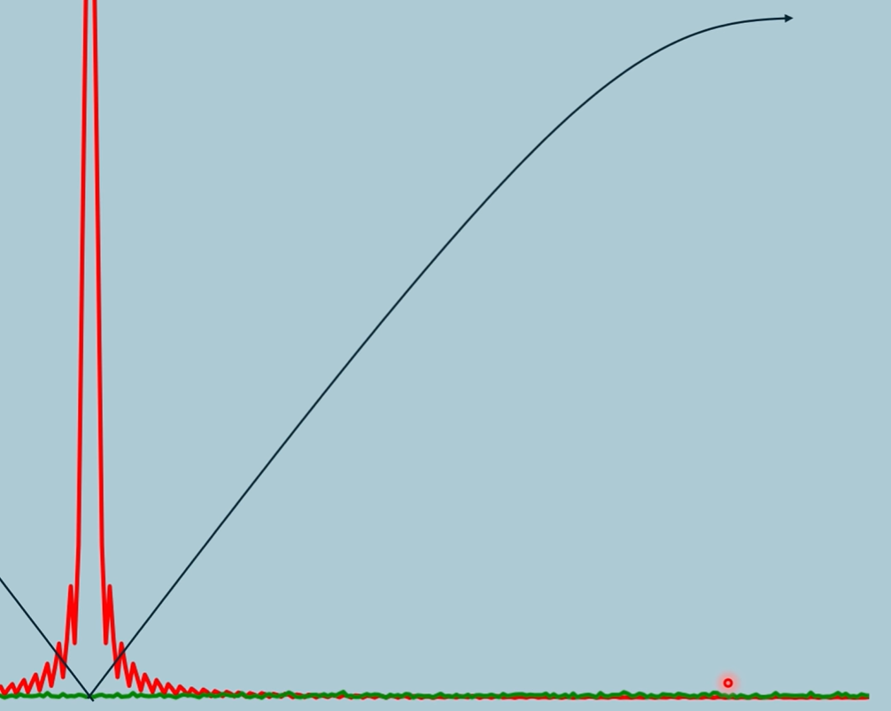
Start with the left diagram. Lambda is the attenuation map for a single projection, and gives values for each x’ position. These values are then back projected across the whole image (values are repeated).

How does the summation work (MUST UNDERSTAND!)?

Imagine you wanted to find the value meue at position x and y. How would you do this? The projection at each angle contributions a value, right? So the attenuation value at an x’ position for each projection angle contributes a value. We use a summation to add all these contributions up.

Video - Filtered Back Projection

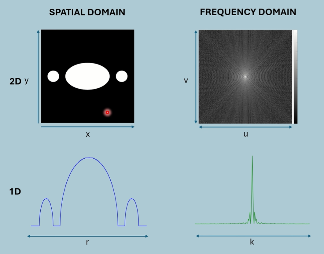
If we look at areas of the image, where there’s little change in the signal over distance, those are low frequency parts of the image. This would be the centre region where there’s high attenuation. As we reach the edge of the low frequency centre, we enter high frequency areas.

A low pass filter will attenuate the high frequency data.

It’s almost as though a non-ideal low pass filter was added to the signal, blurring edges. Fun fact, a blur is a low pass filter.

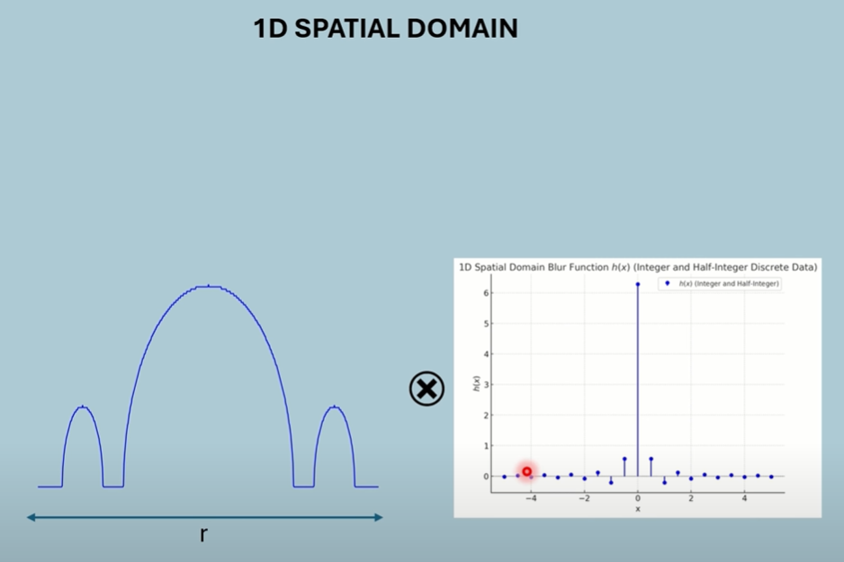
1D Spacial Domain of both object and blur (one projection).

R is distance from centre.

Convolution is computationally demanding in the spacial domain.

Looking at the 1D Spacial Domain, Areas where theres not much change in the image (throughout the centre) is represented by low frequencies. Areas where theres abrupt changes (the dip), consist of high frequencies.

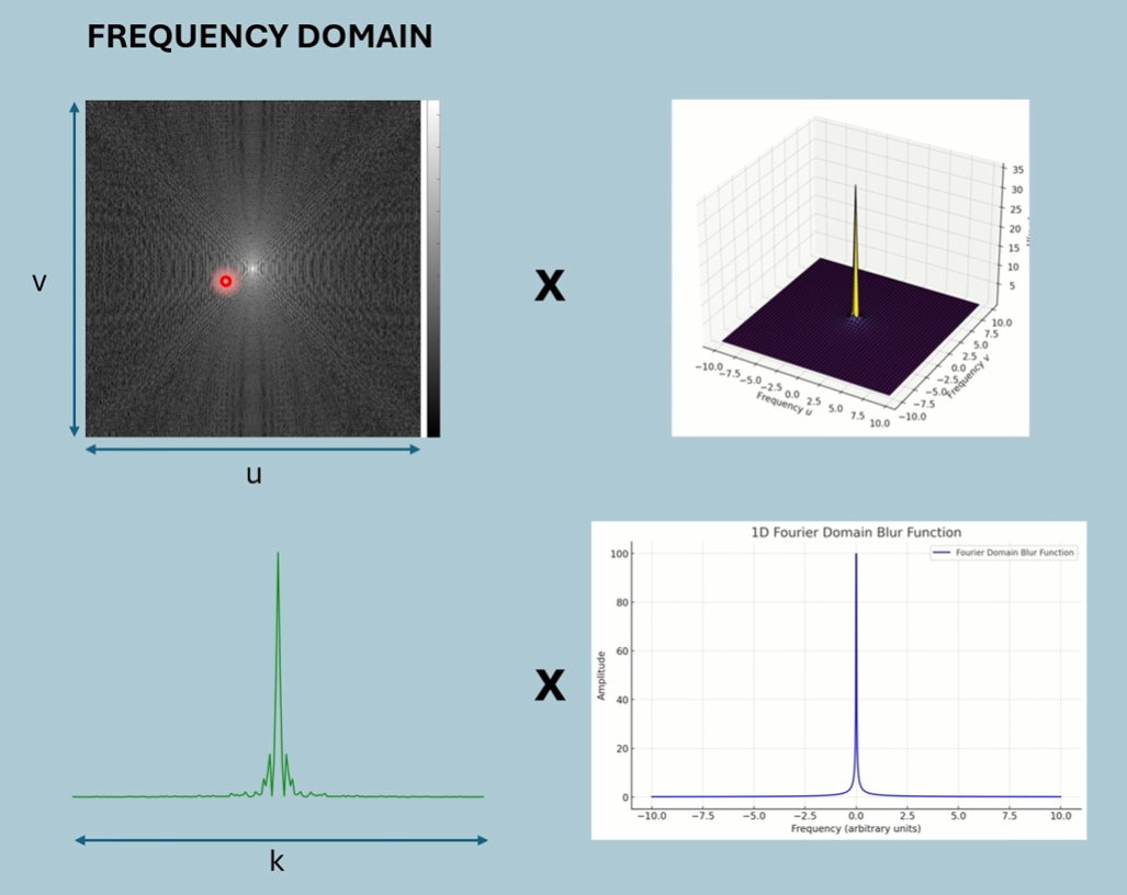
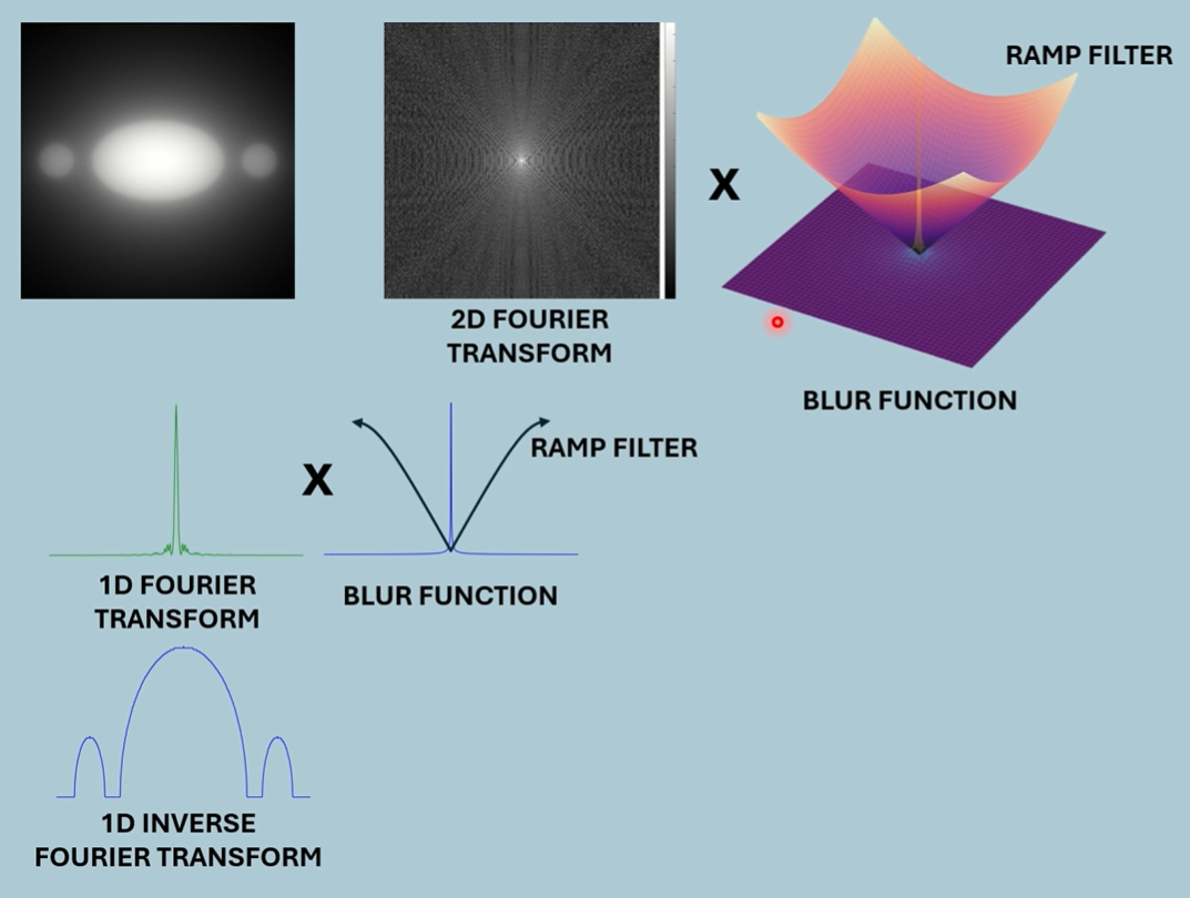
By applying a ramp filter after the blur function to the frequency spectrum, we can raise high frequencies and suppress low, normalising the frequencies.

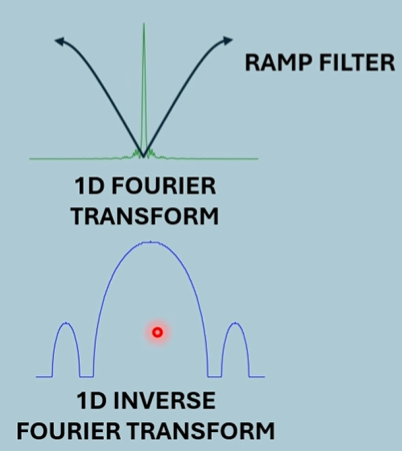
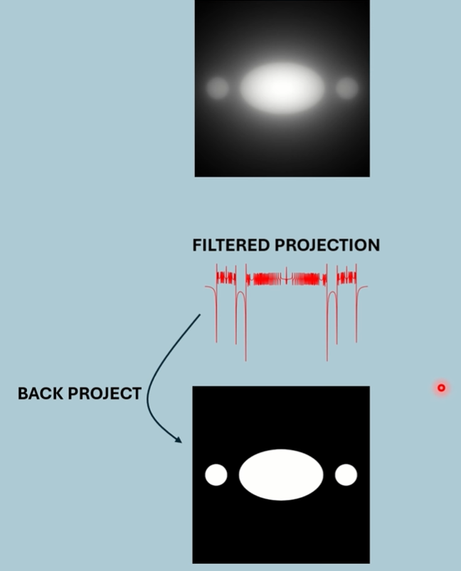
Either we can back project the new 1D spacial, or we can inverse transform the new 2D spectrum.

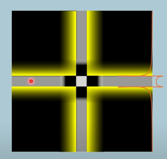
Example

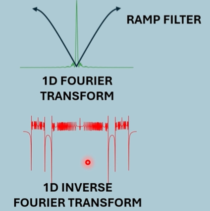
The filtered projection has negative values (zoom in). We back project this and the negative values are now yellow. The positive values are shaded white like usual.

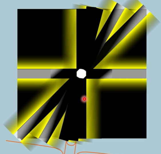
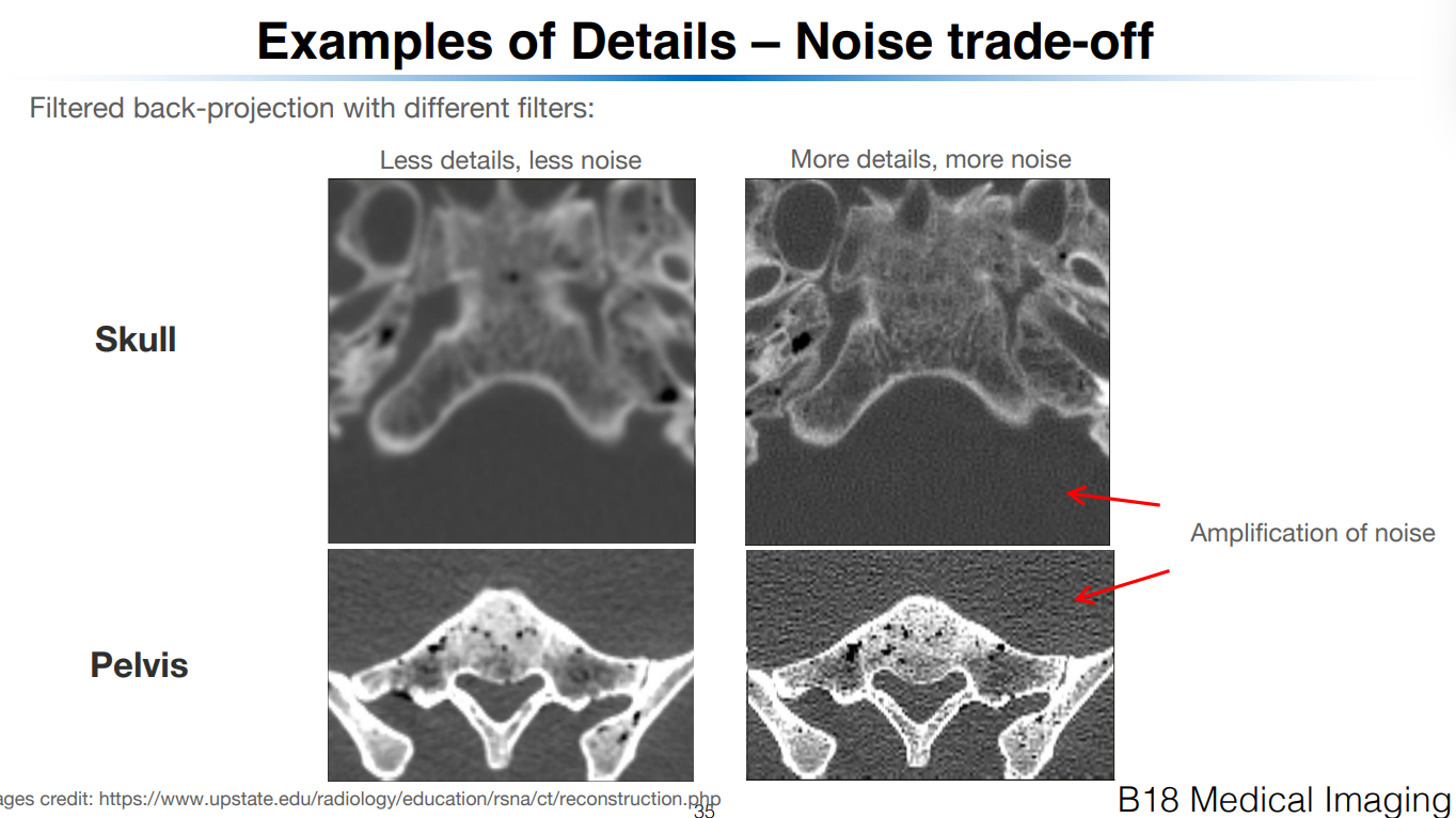
Noise

At high frequencies, the noise is higher than the actual signal

This is why the ramp curves, to keep high freq noise low, but still not enough.

Lectures - Radon Transform

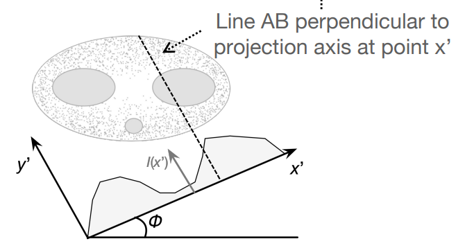
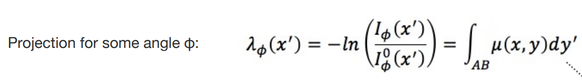
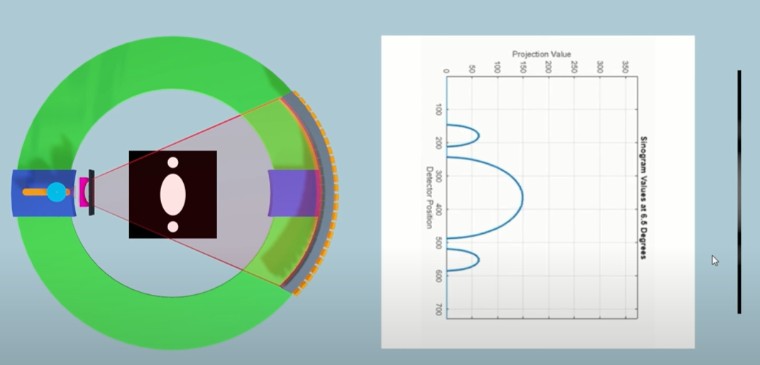
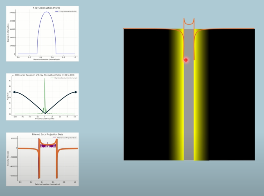
This integral is a single integral on the line x’, along values of y’, giving a single attenuation point on a 1D attenuation map for one projection. This is marked as a red line below on the 1D map. The integral is labelled as line AB (also says dy’), so there’s no need to label x’ in the attenuation function as the integral already defines what line we’re integrating on.

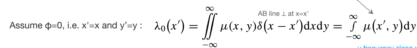
Here is an alternative form of the integral, where projection angle is zero. We start with the double integral over all the attenuation space (x,y), but with a Dirac function, we select only the attenuation values that lie on the line of x’ values (function will be non-zero only when x is part of the line x’). This reduces it down to the previous single integral, but this time we explicitly label in the attenuation function that we only integrate values on the line x’. This is more of a general integral where we integrate over all values of y like normal, but only those corresponding to x’ positions. This again, integrates to a single point on the 1D attenuation map.

1. Line Integral (Single Ray Attenuation):

$\lambda_\phi(x') = \int_{AB} \mu(x, y)\, dy'$

• This integral is for one ray only, the one going through the object along a line perpendicular to the projection axis at detector position $x'$.

• It gives one value of the 1D function $\lambda_\phi(x')$.

Think of this as computing the attenuation for a single X-ray path.

2. The Full Projection:

$\lambda_\phi(x)$

• This entire function is built by evaluating the line integral above for every detector position $x'$.

• So, each $x'$ gives a different integral result, and plotting all of them gives the 1D attenuation curve (the projection).

This is what you see as a line in the sinogram.

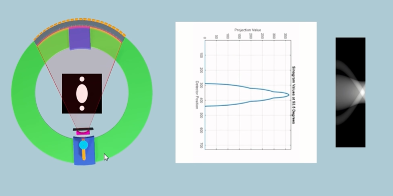
We now take the 1D Fourier Transform of the full projection along an angle = 0.

This is the same as taking a 2D Fourier Transform but with v=0.

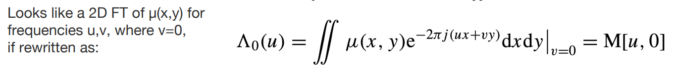
The 1D Fourier Transform of that attenuation map looks like a 2D Fourier Transform but when v = 0.

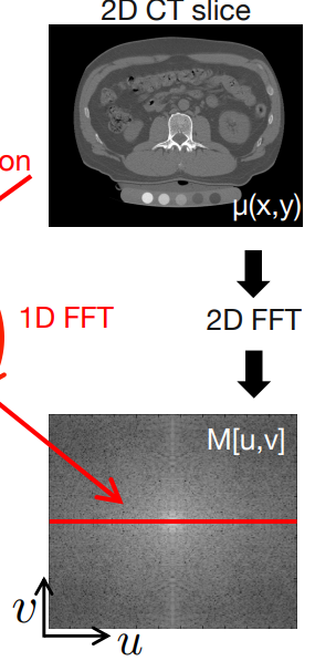
This would correspond to a line of the 2D Fourier Transform of the full CT image, at v=0.

By analogy, we can say the following theorem:

where the projection angle now defines v.

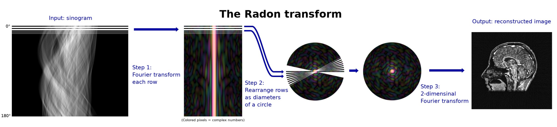
Please note, when v is replaced by the angle, the lines are now in a radial pattern as shown above, where the FT of each line in the sinograph is put onto a circle with different angles. We then inverse 2D Fourier Transform for the CT image.

Lectures + Textbook - Filtered Back Projection

Read the video version first.

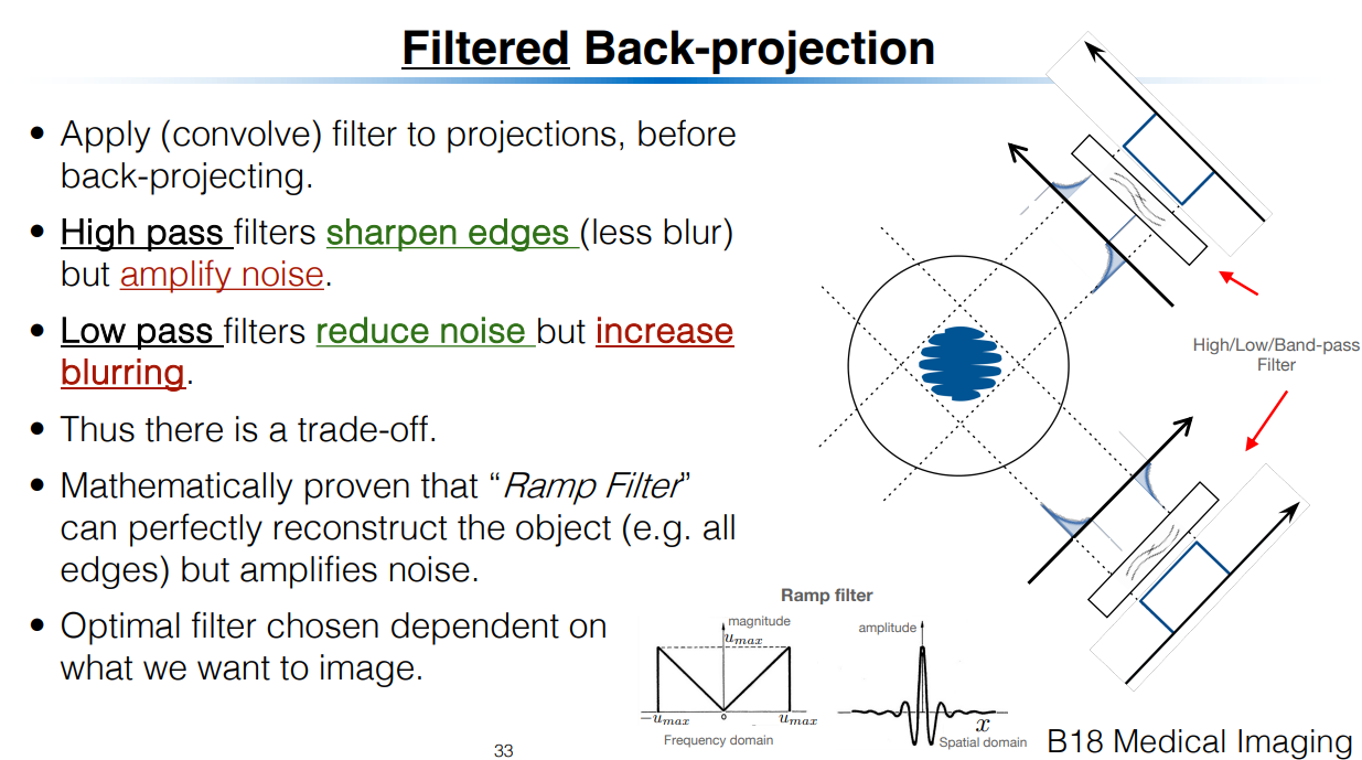
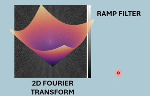
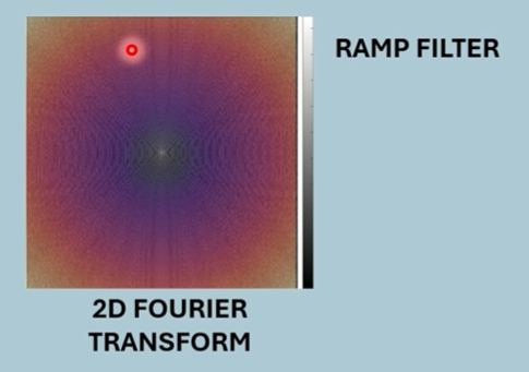
Apply ramp filter in frequency domain before back projecting.

Bottom is orignal 1D spacial attenuation map. The black box represents the ramp filter. The above is the new spacial attenuation map.

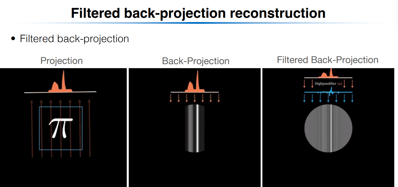
Left is the full attenuation image. Middle is the back projection of a single standard projection. Right is the filtered version of that with the ramp applied.

Maths

Goal of Filtered Back-Projection

We want to reconstruct the original object $\mu(x, y)$ (the spatial distribution of the attenuation coefficient) from the projection data we collected at various angles $\phi$.

🔁 Step 1: Inverse Fourier Transform in Polar Coordinates

From earlier Fourier theory and the Slice-Projection Theorem, we know:

• Each projection $\lambda_\phi(x')$ gives a line in the 2D Fourier transform of $\mu(x, y)$.

• The full 2D Fourier domain of $\mu(x, y)$ is filled by collecting projections at many angles $\phi$.

So the inverse 2D Fourier transform in polar coordinates reconstructs $\mu(x, y)$:

$\mu(x, y) = \int_0^\pi \int_{-\infty}^{\infty} M(\rho, \phi)\, e^{2\pi j\rho(x\cos\phi + y\sin\phi)}\, |\rho|\, d\rho\, d\phi$

Where:

• $M(\rho, \phi)$ is the 2D Fourier transform of $\mu(x, y)$ in polar coordinates.

• $|\rho|$ is a filter (known as the "ramp filter").

🔄 Step 2: Change of Variables

We define:

$x' = x \cos\phi + y \sin\phi$

This is the coordinate along the detector for angle $\phi$. Substituting this simplifies the double integral:

$\mu(x, y) = \int_0^\pi \lambda_\phi^\dagger(x')\, d\phi$

This is the back-projection step: for each projection, we evaluate the function at position $x'$ corresponding to $(x, y)$, and then integrate over all angles.

What does the substitution mean?

Think of the following:

• You're rotating the scanner around the object.

• At each angle $\phi$, the detector measures values along the axis $x'$ (which lies perpendicular to the beam direction).

• The substitution maps a fixed point $(x, y)$ into the rotated detector coordinate $x'$.

So it tells you:

This lets you back-project the correct value for that angle and position.

🔍 Step 2.1: Substitution Maths

Goal:

We want to derive:

$\mu(x, y) = \int_0^\pi \lambda_\phi^\dagger(x')\, d\phi$

from:

$\mu(x, y) = \int_0^\pi \int_{-\infty}^\infty M(\rho, \phi)\, e^{2\pi j\rho(x \cos\phi + y \sin\phi)}\, |\rho|\, d\rho\, d\phi$

Step 1: Identify coordinates in polar frequency space

In this double integral:

• $\rho$: radial frequency

• $\phi$: projection angle

• $M(\rho, \phi)$: the Fourier transform of the object $\mu(x, y)$ in polar coordinates.

The exponential term $e^{2\pi j \rho(x \cos\phi + y \sin\phi)}$ tells you that you're taking the inverse FT along the direction $\phi$ in the spatial domain.

Step 2: Make the substitution

Define a new variable:

$x' = x \cos\phi + y \sin\phi$

This $x'$ represents the position along the detector axis (i.e., the coordinate perpendicular to the X-ray direction at angle $\phi$).

Thus:

$e^{2\pi j \rho(x \cos\phi + y \sin\phi)} = e^{2\pi j \rho x'}$

Now substitute this into Eq. (8.8):

$\mu(x, y) = \int_0^\pi \int_{-\infty}^\infty M(\rho, \phi)\, e^{2\pi j\rho x'}\, |\rho|\, d\rho\, d\phi$

Step 3: Recognize the inner integral as an inverse Fourier transform

Now define a new function:

$\lambda_\phi^\dagger(x') = \int_{-\infty}^\infty M(\rho, \phi)\, |\rho|\, e^{2\pi j\rho x'}\, d\rho$

This is just the inverse Fourier transform of $M(\rho, \phi)\, |\rho|$ with respect to $\rho$, yielding a function of $x'$.

Step 4: Write the full expression using this new variable

Now we substitute the result of the inner integral:

$\mu(x, y) = \int_0^\pi \lambda_\phi^\dagger(x')\, d\phi$

But remember: $x' = x\cos\phi + y\sin\phi$

So more explicitly:

$\mu(x, y) = \int_0^\pi \lambda_\phi^\dagger(x\cos\phi + y\sin\phi)\, d\phi$

This is the filtered back-projection formula.

🔍 Step 3: Define the Filtered Projection

We now define:

$\lambda_\phi^\dagger(x') = \int_{-\infty}^{\infty} M(\rho, \phi)\, |\rho|\, e^{2\pi j \rho x'}\, d\rho$

This is an inverse Fourier transform in $\rho$ of the product $M(\rho, \phi)\, |\rho|$.

To understand this equation, let’s go back to the Slice-Projection Τheorem (taken from slide):

$\Lambda_0(u) = \int \lambda_0(x) e^{-2\pi j u x} dx = \iint \mu(x, y) e^{-2\pi j u x} dxdy = \iint \mu(x, y) e^{-2\pi j (ux + vy)} dxdy|_{v=0} = M[u, 0]$

What would the inverse Fourier version of this look like? Replacing $u$ with $p$, and $x$ with $x’$, and adding filter term $|p|$, our equation is directly analogous as the inverse.

So $\lambda_{\phi}^{\dagger}(x^{\prime})$ is the filtered back projection at a specific angle. It gives you the attenuation value at position $x’$ for a specific projection.

🔁 Step 4: Express as Convolution

The inverse Fourier transform of a product in frequency domain is a convolution in spatial domain. So we write:

$\lambda_\phi^\dagger(x') = \text{iFT}\left(M(\rho, \phi)\, |\rho|\right) = \left[ \text{iFT}(M) \, * \, \text{iFT}(|\rho|) \right](x')$

Using convolution notation $*$, this means:

Then we recall that:

$\Lambda_\phi(\rho) = \text{FT}(\lambda_\phi(x')) \quad \text{(Slice Projection Theorem)}$

So:

$\lambda_\phi^\dagger(x') = \text{iFT}(\Lambda_\phi(\rho) \cdot |\rho|)$

And in convolution form again:

$\lambda_\phi^\dagger(x') = \left[ \lambda_\phi(x') * \text{iFT}(|\rho|) \right]$

🧠 Interpretation Summary:

This means the overall Filtered Back-Projection (FBP) algorithm is:

1. Take each projection $\lambda_\phi(x')$.

2. Filter it by convolving with $\text{iFT}(|\rho|)$ (this is the ramp filter converted to space domain).

3. Back-project the filtered data: For each $(x, y)$, compute $x' = x\cos\phi + y\sin\phi$ (what is the value of $x’$ that contributes to a point x,y), evaluate the filtered projection at that point, and integrate over all $\phi$.

To understand this final stage, go back to simple back-projection and understand the summation term. The summation is equivalent to the integral done here.

Here’s your revised note, now incorporating the practical filters shown in the image:

⚠ Note on the Ramp Filter

The ramp filter $|\rho|$ increases linearly with frequency.

• This boosts high-frequency content, improving edge detail.

• But it also amplifies noise, especially at very high frequencies.

So in practice:

• We band-limit the filter to avoid infinite gain at high frequencies.

• A simple band-limited version is:

  $P(\rho) = \begin{cases} 0 & |\rho| \geq \rho_{\text{max}} \\ |\rho| & |\rho| < \rho_{\text{max}} \end{cases}$

  This sets the filter to zero above a certain cutoff frequency $\rho_{\text{max}}$, and uses the ramp shape below that.

• Other more sophisticated filters exist to reduce noise sensitivity while preserving detail, such as the Shepp-Logan filter:

  $P(\rho) = \left| \left( \frac{2\rho_{\text{max}}}{\pi} \right) \sin\left( \frac{\pi \rho}{2\rho_{\text{max}}} \right) \right|$

  This smooths the transition at high frequencies and offers better rejection of noise while retaining useful detail.

• Additional filters like Hamming and Hann can also be used, typically defined as ramp filters multiplied by window functions to gently suppress high frequencies.

Let me know if you want a visual comparison between these filters or their impact on image quality.

✅ Summary of Full Pipeline

$\boxed{ \mu(x, y) = \int_0^\pi \left[ \lambda_\phi(x') * h(x') \right] \bigg|_{x' = x\cos\phi + y\sin\phi} d\phi }$

Where:

• $\lambda_\phi(x')$ = measured projection

• $h(x') = \text{iFT}(|\rho|)$ = ramp filter in space domain

• $*$ = convolution

• $x' = x\cos\phi + y\sin\phi$ = projection coordinate for location $(x, y)$