Comprehensive Study Notes on Newtonian Forces, Friction, Elasticity, and Biomechanics

Fundamental Definition and Vectorial Nature of Forces

• Physical Definition of Force:

  • A force is a quantitative physical vector quantity that expresses and measures the interaction between two physical systems.
  • A force never exists in isolation; it always represents a mutual interaction acting between two bodies.
  • Every day physical actions—such as pushing, pulling, compressing, or lifting an object—involve the exertion of a force.

• Vector Characteristics of a Force:

  • Magnitude (intensity or modulus).
  • Direction (the line along which the force acts).
  • Sense (the orientation along the direction arrow).
  • Point of application (the specific point on the body where the force is exerted).

• Primary Effects of Forces:

  • Static Effects: Cause elastic or plastic deformation in a body (e.g., a bone subjected to a mechanical load, or the force required for a syringe needle to penetrate human skin).
  • Dynamic Effects: Alter the state of motion of a body by producing an acceleration.

Dynamic Nature of Force: Refuting Common Misconceptions

• Historical Misconception vs. Newtonian Physics:

  • Common intuition (historically formalized by Aristotle) suggested that force is directly proportional to velocity (\text{Force} \n\n\propto v)—asserting that a continuous force is required to maintain constant speed, and that an object stops simply because the driving force ceases.
  • Experimental physics established by Galileo Galilei and Sir Isaac Newton disproved this notion. Friction is the real agent that causes moving objects to decelerate and come to rest.
  • In the absence of resistive forces, no net force is required to keep a body moving at a constant velocity.

• Fundamental Relationship:

  • A net force is required to change the velocity of a body (i.e., to cause acceleration or deceleration).
  • The correct mathematical relation is:   $\text{Force} \propto \text{acceleration}$$\vec{F} = m \mathbf{a}$
  • Whenever a change in the state of motion of a body is observed, a net force must be identified as the underlying cause.

Fundamental Classification of Forces

• Action-at-a-Distance Forces:

  • Forces that act without physical contact between objects. Many of these forces are conservative.
  • Gravitational Force: Universal attractive interaction between masses.
  • Electrostatic Force: Interaction between electric charges.

• Contact Forces:

  • Forces that result from direct macroscopic contact between physical surfaces or bodies.
  • Friction Force: Dissipative force opposing relative sliding or motion.
  • Tension Force: Force transmitted through stretched ropes, cords, or cables.
  • Fluid Pressure: Force exerted by fluids per unit surface area.

Gravitational Force and Weight Force

• Newton's Law of Universal Gravitation:

  • Any two point masses $m_1$ and $m_2$ separated by a distance $r$ attract each other with a force directly proportional to the product of their masses and inversely proportional to the square of the distance between them:   $F = G \times \frac{m_1 \times m_2}{r^2}$
  • Universal Gravitational Constant: $G = 6.67428 \times 10^{-11}\,\text{m}^3\,\text{kg}^{-1}\,\text{s}^{-2}$.

• Gravitational Acceleration at Earth's Surface:

  • Setting $m_1 = M_{\text{Earth}}$ (mass of the Earth) and $r = R_{\text{Earth}}$ (mean radius of the Earth):   $F = \left(G \times \frac{M_{\text{Earth}}}{R_{\text{Earth}}^2}\right) \times m = g \times m$
  • Acceleration due to gravity at Earth's surface:   $g = \frac{G \times M_{\text{Earth}}}{R_{\text{Earth}}^2} = 9.81\,\text{m/s}^2$

• Weight Force Definition:

  • The weight force $\vec{F}_g$ (or $\vec{P}$) acting on a mass $m$ is the gravitational attraction exerted on it by Earth:   $\vec{F}_g = \vec{P} = m\mathbf{g}$
  • Direction and Sense: Pointed vertically downward, directed toward the center of Earth.
  • Geoid Effect: Earth is an oblate spheroid (geoid) rather than a perfect sphere. The Earth's radius $R$ is larger at the Equator than at the Poles. Consequently, gravitational acceleration $g$ is slightly smaller at the Equator compared to the Poles.

• Units and Dimensional Analysis:

  • SI Unit of Force: Newton ($\text{N}$).   $1\,\text{N} = 1\,\text{kg} \times 1\,\text{m/s}^2$
  • A mass of $1\,\text{kg}$ subjected to standard gravity ($g \approx 9.81\,\text{m/s}^2 \approx 10\,\text{m/s}^2$) experiences a weight force of approximately $9.81\,\text{N}$ (or $\approx 10\,\text{N}$).
  • Practical System Unit: Kilogram-force ($\text{kgp}$ or $\text{kg}_f$):   $1\,\text{kgp} = 1\,\text{kg} \times g = 9.81\,\text{N} \approx 10\,\text{N}$

• Distinction Between Mass and Weight:

  • Mass ($m$): An intrinsic scalar property of matter, measured in kilograms ($\text{kg}$), which remains constant everywhere in the universe.
  • Weight ($\vec{F}_g$): A force dependent on local gravitational acceleration $g$.
  • Free-Fall Kinematics (in vacuum with $y_0 = H$ and $v_0 = 0$):$v(t) = -g \times t$$y(t) = H - \frac{g}{2} \times t^2$
  • Earth vs. Moon Comparison:
  • On Earth ($g \approx 9.81\,\text{m/s}^2$): A mass $m = 1\,\text{kg}$ has $F_g = 9.8\,\text{N}$; a mass $m = 10\,\text{kg}$ has $F_g = 98\,\text{N}$.
  • On the Moon: Gravitational acceleration is roughly one-sixth of Earth's gravity ($g_{\text{Moon}} \approx \frac{1}{6} g_{\text{Earth}}$). A body's weight on the Moon drops to one-sixth of its Earth weight, while its mass remains entirely unchanged.

• Numerical Examples and Order-of-Magnitude Calculations:

  • Example 1 (Weight Estimation):
  • Problem: A backpack has a mass $m = 8\,\text{kg}$. What is its approximate weight?
  • Calculation: $F_g = m \times a = 8\,\text{kg} \times 9.81\,\text{m/s}^2 \approx 8 \times 10 = 80\,\text{N}$.
  • Example 2 (Gravitational Attraction Between Small Spheres):
  • Problem: Two spheres of mass $m_1 = m_2 = 5\,\text{kg}$ are placed at a distance $r = 0.5\,\text{m}$. Estimate the order of magnitude of their mutual gravitational force ($G = 6.7 \times 10^{-11}\,\text{N}\,\text{m}^2\,\text{kg}^{-2}$).
  • Calculation:     $F = G \times \frac{m_1 \times m_2}{r^2} \approx \left(6.7 \times 10^{-11}\right) \times \frac{5 \times 5}{(0.5)^2} = 6.7 \times 10^{-11} \times \frac{25}{0.25} = 6.7 \times 10^{-9}\,\text{N} \approx 10^{-8}\,\text{N}$
  • Resulting order of magnitude: $10^{-8}\,\text{N}$.

Electrostatic Force and Relative Strength Comparison

• Coulomb's Law:

  • Calculates the magnitude of the electrostatic attraction or repulsion between two point charges $q_1$ and $q_2$ separated by distance $d$:   $F = k \times \frac{q_1 \times q_2}{d^2}$
  • Units: $F$ in Newtons ($\text{N}$), charges in Coulombs ($\text{C}$), distance in meters ($\text{m}$).
  • Electrostatic Proportionality Constant:$k = \frac{1}{4\pi \varepsilon_0} = \frac{\mu_0 \times c^2}{4\pi} = 8.99 \times 10^9\,\text{N}\,\text{m}^2\,\text{C}^{-2}$

• Comparison Between Electrostatic and Gravitational Constants:

  • $k = 8.99 \times 10^9\,\text{N}\,\text{m}^2\,\text{C}^{-2}$
  • $G = 6.7 \times 10^{-11}\,\text{N}\,\text{m}^2\,\text{kg}^{-2}$
  • Since $k \gg G$, electrostatic forces completely dominate over gravitational forces at atomic and molecular scales. In the presence of electrostatic interactions, gravitational forces between charged particles are negligible.

Normal Contact Force (Constraint Force)

• Definition and Mechanism:

  • The normal force $\vec{F}_N$ (or $\vec{N}$) is the contact force exerted perpendicular (normal) to the surface of contact.
  • It acts as a mechanical constraint force that prevents a body from penetrating or falling through a solid support surface.

• Equilibrium on a Horizontal Plane:

  • For a stationary body resting on a flat horizontal plane ($\mathbf{a} = 0$):   $\vec{F}_N + \vec{F}_g = 0$$F_N - m\mathbf{g} = 0 \implies F_N = m\mathbf{g}$

Friction Forces Between Solid Surfaces

• Microscopic Origin:

  • Friction arises from electrostatic interactions and physical interlocking between microscopic irregularities (asperities) of contacting materials.
  • Biological systems utilize special lubricants to reduce friction (e.g., synovial fluid in human joint cavities).

• Classification of Friction Forces:

  • Static Friction ($F_s$): Prevents the initiation of relative sliding motion between stationary contacting surfaces. It increases proportionally with the applied force up to a maximum threshold value, at which point the static bond breaks.
  • Kinetic (Dynamic) Sliding Friction ($F_k$): Resists continuous relative sliding motion between two surfaces in contact.
  • Rolling Friction (Dynamic Volvente): Resists the rolling motion of spherical or cylindrical objects (such as wheels, spheres, or wheelchair castors) across a surface. Rolling friction is generally much weaker than kinetic sliding friction because the instantaneous surface area of contact is substantially smaller.

• General Mathematical Formulation:$F_a = \mu_a \times F_{\perp} = \mu_a \times F_N$

  • $F_a$: Friction force acting parallel to the surface, directly opposing motion or the attempted direction of motion.
  • $\mu_a$: Dimensionless coefficient of friction characteristic of the pair of materials.
  • $F_{\perp}$ (or $F_N$): Normal pressing force acting perpendicular to the contact plane.

• Direction and Vector Orientation Clarification:

  • The normal force $F_N$ acts perpendicular to the surface.
  • Friction ($F_s$ or $F_k$) acts parallel to the surface, oriented opposite to the motion (or impending motion).
  • The equation $F_a = \mu_a \times F_N$ scales the magnitude only; the two forces are mutually perpendicular vectors.

• Properties of Dynamic Friction:

  • Independent of the macroscopically visible surface contact area.
  • Independent of relative sliding speed over ordinary ranges.
  • Directly proportional to the normal force $F_N$
  • Coefficient relationship: For any given pair of materials, the kinetic friction coefficient $\mu_k$ is strictly smaller than the static friction coefficient $\mu_s$ ($\mu_k < \mu_s$).

• Self-Adjusting Nature of Static Friction:

  • The maximum threshold of static friction is $F_{s,\max} = \mu_s \times F_N$.
  • If the applied pushing force $F_{\text{applied}}$ is less than $F_{s,\max}$, the static friction force adapts to exactly match the applied force: $F_s = F_{\text{applied}}$, keeping the body at rest.
  • Motion starts only when $F_{\text{applied}} > F_{s,\max}$. Once motion begins, the opposing force drops immediately to the kinetic friction value $F_k = \mu_k \times F_N$

• Standard Coefficients of Friction ($\mu_s$ and $\mu_k$):

• Practical Worked Examples:
  • Example 1 (Threshold force required to initiate movement of $1\,\text{kg}$ mass):
  • For Wood on Wood ($m = 1\,\text{kg}$, $\mu_s = 0.4$):       $F_{\text{threshold}} = \mu_s \times m\mathbf{g} = 0.4 \times 1\,\text{kg} \times 9.8\,\text{m/s}^2 \approx 4\,\text{N}$
  • For Ice on Ice ($m = 1\,\text{kg}$, $\mu_s = 0.1$):       $F_{\text{threshold}} = \mu_s \times m\mathbf{g} = 0.1 \times 1\,\text{kg} \times 9.8\,\text{m/s}^2 \approx 1\,\text{N}$
  • Example 2 (Static Friction Adaptation):
  • A block of mass $m = 10\,\text{kg}$ rests on a horizontal plane ($N = 100\,\text{N}$). The static coefficient is $\mu_s = 0.4$. A horizontal force of $20\,\text{N}$ is applied.
  • Maximum potential static friction: $F_{s,\max} = 0.4 \times 10\,\text{kg} \times 10\,\text{m/s}^2 = 40\,\text{N}$.
  • Since $20\,\text{N} < 40\,\text{N}$, the block remains motionless, and the active static friction force is exactly $20\,\text{N}$.
  • Example 3 (Crate Motion Thresholds):
  • A crate weighs $200\,\text{N}$ on a horizontal floor with $\mu_s = 0.40$ and $\mu_k = 0.30$.
  • Minimum force to start motion: $F_{s,\max} = \mu_s \times F_N = 0.40 \times 200\,\text{N} = 80\,\text{N}$.
  • Force required to maintain constant sliding velocity: $F_k = \mu_k \times F_N = 0.30 \times 200\,\text{N} = 60\,\text{N}$.

Analysis of Motion on an Inclined Plane

• Force Decomposition:

  • Consider an object of mass $m$ on a plane inclined at an angle $\theta$ to the horizontal:
  • Perpendicular component of gravity: $F_{\perp} = m\mathbf{g} \times \cos(\theta)$, balanced by the normal force $F_N = m\mathbf{g} \times \cos(\theta)$.
  • Parallel component of gravity (driving force down the slope): $F_{\parallel} = m\mathbf{g} \times \sin(\theta)$.
  • Opposing static friction force: $F_a$.

• Static Equilibrium on an Inclined Plane:

  • Condition to prevent sliding down the ramp:   $F_a = F_{\parallel} = m\mathbf{g} \times \sin(\theta)$
  • Maximum available static friction force:   $F_{s,\max} = \mu_s \times F_N = \mu_s \times m\mathbf{g} \times \cos(\theta)$
  • Critical threshold condition for slipping:   $m\mathbf{g} \times \sin(\theta) = \mu_s \times m\mathbf{g} \times \cos(\theta) \implies \mu_s = \frac{\sin(\theta)}{\cos(\theta)} = \tan(\theta)$

• Worked Inclined Plane Problems:

  • Problem 1 (Actual static friction calculation):
  • A $10\,\text{kg}$ block rests on a $30^\circ$ slope with $\mu_s = 0.8$. What is the actual static friction force acting on it?
  • $F_{\parallel} = m\mathbf{g} \times \sin(30^\circ) \approx 10\,\text{kg} \times 10\,\text{m/s}^2 \times 0.5 = 50\,\text{N}$.
  • $F_{s,\max} = \mu_s \times m\mathbf{g} \times \cos(30^\circ) = 0.8 \times 100 \times 0.866 = 69.3\,\text{N}$.
  • Since $50\,\text{N} < 69.3\,\text{N}$, the block does not slide, and the active static friction force is $50\,\text{N}$.
  • Problem 2 (Minimum coefficient for equilibrium):
  • What minimum static friction coefficient $\mu_s$ prevents a block from sliding down a $30^\circ$ incline?
  • $\mu_s = \tan(30^\circ) = \frac{\sin(30^\circ)}{\cos(30^\circ)} = \frac{0.5}{0.866} \approx 0.58$

Viscous Friction in Biological and Fluid Dynamics

• Low Velocity Fluid Resistance (Stokes' Law):

  • Describes the viscous drag force $F_a$ acting on a small spherical body moving at low velocity through a laminar fluid:   $F_a = 6\pi \times \eta \times r \times v$
  • $r$: Radius of the sphere (m).
  • $\eta$: Dynamic viscosity of the fluid ($\text{N}\,\text{s}\,\text{m}^{-2}$ or $\text{Pa}\,\text{s}$).
  • $v$: Velocity relative to the fluid ($\text{m/s}$).
  • Dimensional Verification: $\left(\text{N}\,\text{s}\,\text{m}^{-2}\right) \times \text{m} \times \left(\text{m/s}\right) = \text{N}$.

• High Velocity Aerodynamic Drag:

  • When object velocity is high and turbulence occurs, resistive force scales quadratically with speed:   $F_a = \frac{1}{2} \times c_x \times \rho \times S \times v^2$
  • $c_x$: Aerodynamic drag coefficient (dimensionless shape-dependent index).
  • $\rho$: Fluid density ($\text{kg/m}^3$).
  • $S$: Cross-sectional frontal area ($\text{m}^2$).
  • $v$: Velocity relative to the fluid ($\text{m/s}$).
  • Dimensional Verification: $\left(\text{kg/m}^3\right) \times \text{m}^2 \times \left(\text{m}^2/\text{s}^2\right) = \text{kg}\,\text{m/s}^2 = \text{N}$.

Tension Forces and Pulley Systems

• Ideal Rope Properties:

  • Massless ($m \approx 0$).
  • Inextensible (fixed length under stress).
  • Incompressible (only transmits tensile pulling forces).
  • Transmits mechanical force along its entire length from one end to the other, causing linked bodies to move together with identical acceleration magnitude $a$

• Ideal Pulleys:

  • A massless, fixed pivot point around which an ideal rope redirects its vector direction while keeping tension magnitude $T$ identical across all segments on both sides.
  • Clinical Application: Mechanical traction of injured human limbs via arrangements of cords and pulleys. The pulley changes the direction of pulling force without altering its magnitude ($P = T$).

• Centripetal Tension in Rotational Motion:

  • Tension in a tethered system provides the required centripetal acceleration $a_c$ to maintain circular orbital motion:   $T = m \times a_c$

Elastic Forces, Hooke's Law, and Harmonic Motion

• Hooke's Law for Ideal Springs:

  • When an elastic body or spring undergoes displacement $\Delta x = x - x_0$ from its resting length $x_0$, a restoring force arises that opposes deformation:   $F_{\text{el}} = -k \times \Delta x = -k \times (x - l_0)$
  • $k$: Elastic spring constant ($\text{N/m}$).
  • The negative sign signifies that the restoring force acts opposite to displacement.

• Differential Equation of Simple Harmonic Motion:

  • Applying Newton's Second Law to a spring-mass system ($l_0 = 0$):   $m \times a = -k \times x$
  • Expressing acceleration as the second derivative of position with respect to time ($a = \frac{d^2 x}{d t^2}$):   $\frac{d^2 x}{d t^2} = -\left(\frac{k}{m}\right) \times x = -\omega^2 \times x$
  • Solutions to this differential equation take the general sinusoidal form of simple harmonic motion:   $x(t) = A \times \sin(\omega t + \varphi)$
  • Angular frequency $\omega$, frequency $f$, and period $T$:   $\omega = 2\pi f = \frac{2\pi}{T} = \sqrt{\frac{k}{m}}$

• Numerical Practice Example:

  • Problem: An ideal spring with elastic constant $k = 200\,\text{N/m}$ is stretched by $\Delta x = 3\,\text{cm}$ ($0.03\,\text{m}$). Calculate the magnitude of the restoring force.
  • Calculation: $F = k \times x = 200\,\text{N/m} \times 3 \times 10^{-2}\,\text{m} = 6\,\text{N}$.

Continuum Mechanics and Biomechanical Elasticity of Tissues

• Stress and Strain Definitions:

  • Stress (Specific Load, $\tau$): The deforming force applied per unit cross-sectional area:     $\tau = \frac{F}{S} \quad \left[\text{N/m}^2 \text{ or } \text{Pa}\right]$
  • Strain (Relative Deformation, $\gamma$): Fractional change in length relative to initial resting length:     $\gamma = \frac{\Delta l}{l_0} \quad \left[\text{dimensionless}\right]$

• Deformation Phases of Biological Materials:

  • Elastic Region: Linear behavior where stress is directly proportional to strain. Upon removing the load, the body returns completely to its original shape.
  • Inelastic / Plastic Region: Occurs once stress exceeds the critical yield point (carico specifico di snervamento). Permanent irreversible deformation remains after removing the load.
  • Fracture / Breaking Point: The ultimate terminal stress $\Sigma$ at which material structural failure occurs.

• Young's Modulus ($E$):

  • Within the linear elastic regime, Hooke's generalized law holds:   $\frac{\tau}{\gamma} = E \implies \tau = E \times \gamma$
  • Young's modulus $E$ ($\text{Pa}$ or $\text{N/m}^2$) quantifies material stiffness and depends strictly on the material composition and type of stress (tensile vs. compressive).

• Transverse Contraction and Poisson's Ratio ($P$):

  • When a continuous body is stretched longitudinally, it narrows laterally. The fractional lateral dimensional change $\Delta s$ relates to longitudinal strain $\Delta l$ via Poisson's ratio $P$:   $\Delta s = P \times \Delta l$

• Mechanical Properties of Biological Tissues vs. Biomaterials:

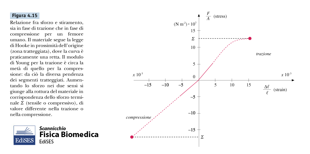
• Biomechanical Behavior of Human Femur Under Stress:
  • The human femur obeys Hooke's linear relation near the origin (dashed regime).
  • Tension vs. Compression Asymmetry: Young's modulus for tensile loading is approximately half of that observed for compressive loading ($E_{\text{tension}} \approx \frac{1}{2} E_{\text{compression}}$). This is reflected by differing initial linear slopes.
  • Ultimate breaking stress $\Sigma$ also differs significantly between tension and compression.

• Torsional Moments and Bone Spiral Fractures:
  • Internal torsional moment opposes external applied torque $\mathbf{T} = \mathbf{F} \wedge \mathbf{R}$ to maintain section equilibrium.
  • Excessive rotational torque applied across long bones (e.g., the tibia) produces classic helical torsional fractures, known as spiral fractures.

Muscle Forces and Musculoskeletal Mechanics

• Muscular Force Significance:

  • Muscle forces represent the primary internal active forces in physiological and biomechanical applications.

• Structural Hierarchy of Striated Skeletal Muscle:

  • Whole Muscle \n\n\rightarrow Muscular Fiber Bundles (muscle cells) \n\n\rightarrow Individual Muscle Fiber (Myofiber) \n\n\rightarrow Myofibril \n\n\rightarrow Sarcomere (the functional contractile unit bounded by Z-lines, featuring H-zone, I-bands, and A-bands containing sliding actin and myosin filaments).

• Musculoskeletal Levers and Antagonistic Action:
  • Skeletal muscles attach to bones via collagenous tendons across biological joints.
  • Muscle contraction exerts tensile forces that generate rotational moments around joint axes.
  • Movements are coordinated in opposing pairs: agonist muscles (which produce a specific joint rotation) work opposite antagonist muscles (which produce reverse rotation).

Summary of Key Mechanical Force Equations

• Universal Gravitation:$F = G \times \frac{m_1 \times m_2}{r^2}$

• Weight Force:$P = m\mathbf{g}$

• Friction Between Solid Surfaces:$F_a = \mu_a \times F_N$

• Viscous Friction in Fluids:

  • Low velocity (Stokes): $F_a = 6\pi \times \eta \times r \times v$
  • High velocity: $F_a = \frac{1}{2} \times c_x \times \rho \times S \times v^2$

• Hooke's Law for Springs:$F = -k \times \Delta x$

• Generalized Elasticity Law for Continuous Media:$\frac{\tau}{\gamma} = E$$\frac{F/S}{\Delta l / l_0} = E$