ECON201
Law of demand: Price and quantity demanded of any good and service are inversely related to each other
Shifts along demand curve caused by changes in price only
Shifts in demand curve caused by:
- Price of substitutes
- Price of complements
- Income
- Preferences
- Number of consumers
- Future expectations
Law of supply: Price and quantity supplied of any good and service are generally positively related to each other
Quantity and price general positive relationship due to law of diminishing marginal production leading to increasing marginal costs
Shifts along supply curve caused by changes in price only
Shifts in supply curve cause by:
- Price of other goods
- Production costs
- Technology
- Number of sellers
- Future expectations
The magnitude of changes in equilibrium price and quantity are impacted by:
- Size of shift
- Slope of curves related to price elasticities
As you move down a demand or supply curve, it become less elastic (more inelastic) - Eventually perfectly inelastic at the horizontal axis
Market efficiency sees:
- Both CS and PS maximised
- DWL = 0
- Last unit transacted MB = MC
Taxes, price ceilings and price floors create DWL and market inefficiencies
Producer subsidies create DWL but increase PS at a cost to the government
Consumer Behaviour Introduction
How do consumers make purchases?
Ultimately, consumers are assumed to ‘optimise’ their utility given scarce resources
Consumer theory is the basis for the ‘demand’ side of the supply and demand model
Consumer Preferences & The Concept of Utility
Consumers are rational and ‘optimise’ consumption decisions given scarce resources
Four assumptions about consumer preferences:
- Completeness and Rankability
Consumers can compare bundles of goods and rank them based on preference
- For most goods, more is better than less
Non-satiation and free disposal → MU > 0
Preferences are strongly monotonic: A basket with more of at least one good and no less of the other good is preferred to the original basket
- Transitivity
Imposes logical consistency on preferences
Consumers make choices that are consistent with each other e.g. if A > B and B > E then A > E
- The more a consumer has of a particular good, the less they are willing to give up something else to get even more of that good
This assumes consumers like variety
Principle of diminishing marginal utility
Utility is a measure of how ‘satisfied’ consumers are
- A measure of happiness or well-being
- It is not a measure of consumer income
A utility function mathematically describes the relationship between a consumers actual consumption and their level of well-being
- Represents consumer preferences
- Can take a variety of mathematical forms
- Haves to conform to the four assumptions about preferences
Utility with a single good
The marginal utility (MU) is the slope of the total utility function
Diminishing Marginal Utility: After some point, increased consumption of a good sees the marginal utility of that good begin to fall
As the quantity consumed increases, the marginal utility gained from consuming each additional good falls
Marginal Utility: The additional utility a consumer receives from an additional unit of a good or service
Comparing Consumption Outcomes
The ‘rules’ for utility allow only for an ordinal ranking of consumption bundles
- An ordinal ranking implies bundles can be ranked from best to worst
- A cardinal ranking would allow a person to determine how much better one bundle is, compared to another
- There is no real-world measure of how much more a consumer likes the bundle of goods A to the bundle of goods B
Indifference Curves
Ordinal rankings mean we care about relative outcomes
A consumer is indifferent between bundles is when they derive the same utility level from two or more bundles
An indifference curve plots out all of the consumption bundles that provide a consumer with the same level of utility or satisfaction
Characteristics of Indifference Curves (from the four assumptions about consumer preferences):
- They can be drawn - completeness and rankability
- Curves further from the origin represent higher utility - more is better
- Curves never cross - transitivity
- Convex to the origin - consumers like variety + diminishing marginal utility
Curves are:
- Parallel
- Downward sloping
- As you move down the gradient diminishes
A consumers indifference curves cannot cross
Tradeoffs: Initially consumers consume greater quantities of one good compared to another, however this can be compensated by consuming a greater amount of the latter good and a lesser amount of the first good to leave utility unchanged.
E.g. as apartment size increases, Jo is less willing to trade off the number of friends for additional apartment size → diminishing marginal returns
The Marginal Rate of Substitution (MRS)
Indifference curves describe tradeoffs
→ How much of one good are you willing to give up for one more unit of another good?
→ The slope of the indifference curve captures this tradeoff - Referred to as the marginal rate of substitution
Describes the rate at which one is willing to trade off or substitute exactly 1 unit of good X for more of good Y, and be equally well off
As you move down an indifference curve, you experience a diminishing marginal rate of substitution
Along an indifference curve, the change in utility is zero
The law of diminishing utility dictates that the higher quantity consumed of something, the less marginal utility is gained from consumption and vice versa.
Therefore, the marginal rate of substitution decreases as you move down an indifference curve
The MRS between two goods is equal to the inverse of the goods marginal utilities
- Steeper curves imply the consumer is willing to give up a lot of Y to get one unit of X, or could trade 1 unit of X for a lot of good Y
- Flatter curves imply the consumer would require a large increase in good X to give up one Y, or could trade 1 unit of good Y for a lot of good X
The Curvature of Indifference Curves: Substitutes and Complements
The shape of indifference curves reveals information about the relationship between products.
- Relatively straight indifference curves - goods that are more easily substitutable for one another
- e.g. Decaf latte for decaf coffee
- Indifference curves that are more convex to the origin - goods that are more complementary to one another
- e.g. tortilla chips for guacamole
Perfect substitutes: Goods that the consumer will trade at a fixed rate and receive the same level of utility (MRS is constant)
Perfect complements: Goods that the consumer must consume in a fixed proportion
e.g. Tortilla chips in 3-oz and 12-oz proportions - would be willing to trade 4 for 1 no matter the quantity so MRS is constant in this case
e.g. left and right shoes
The same consumer can have indifference curves with different shapes
Initially for low levels of utility (Ua), bananas and strawberries may be substitutes
As utility increases (Ub), consumers might prefer a variety of fruit in their diet more than initially
Consumers Income and the Budget Constraint
Could be visualised as a consumption possibility frontier - similar to PPF
The budget constraint is a curve that describes the entire set of consumption bundles a consumer can purchase when spending all of their income
It is generally plotted alongside indifference curves.
For two goods: Income = PxQx + PyQy
Gradient = -Px / Py
Factors that Affect the Budget Constraints Position
The slope and position of the budget constraint are a function of two factors: income and relative prices
- Change in income shifts the budget constraint by changing the intercepts - moves parallel
- Change in the price of one good pivots the budget constraint by changing the slope - only parallel if price change is proportionate
Consumer Optimisation Problem
- Indifference curves - utility and describe consumer preferences
- Budget constraint describes which bundles are feasible
- Combining concepts allows the understanding of consumer choices
Consumers face a constrained optimisation problem → Maximise utility, subject to income and market prices
Bundle A slope of the budget line = slope of the indifference curve
Consumer equalises marginal utility per dollar spent is across all products
Getting more utility per dollar from X, therefore you should consume more of good X until the MUx decreases so that the ratio is equal again 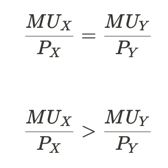
Two consumers facing the same income and the same prices but have different preferences will still have the same MRS at their optimal bundles due to the same ratio of prices
Interior Solution: A utility maximising bundle that contains positive quantities of both goods
Depending on consumers preferences and relative prices, in some cases a consumer will not want to spend any of their money on a good
Corner solution: a utility-maximising bundle located at the ‘corner’ of the budget constraint where the consumer purchases only one of two goods
Perfect substitutes:
Perfect complements:
Indeterminate budget constraint:
Individual and Market Demand
Income Changes & Individual Consumption Choices
→ Links consumer decision framework with individual and market demand
The income effect - Change in a consumer’s consumption choices due to a change in the consumer’s income (or purchasing power), holding relative prices constant
It depends on the good whether higher income is associated with higher consumption of goods
Normal good - higher income is associated with rising consumption e.g. vacations and basketball tickets
Necessity goods: normal goods for which income elasticity is between 0 and 1 e.g. water consumption, electricity, clothing etc.
10% income increase / 3% quantity demanded increase = Ep = 0.3
Luxury goods: normal goods for which income elasticity is greater than 1 e.g. vacation homes, jewelry, expensive steaks, etc.
10% income increase / 13% quantity demanded increase = Ep = 1.3
Inferior good - higher income is associated with falling consumption e.g. lower quality goods, income rise sees switch away to higher quality goods
Income expansion path: a curve that connects a consumer’s optimal bundles at each income level
- If both goods are normal goods, the path is positively sloped
- If the slope of the income path is negative, one of the goods is an inferior good
Engel curve: Shows the consumption-income relationship
- Shows the relationship between quantity of a good consumed and a consumer’s income
- If the Engel curve has a positive slope, the good is a normal good at that income level
- If the Engel curve has a negative slope, the good is an inferior good at that income level
Engel curve compares income to one good
Deriving demand curve:
Relates to law of demand and substitution effect (consumers swap to cheaper good as price decreases)
First part of demand curve is elastic (price drop causes greater increase in demand), second part is inelastic (price drop causes lesser increase in demand)
Area under demand curve represents consumers total utility
Income and Substitution Effects
When the price of a good changes relative to another, two things happen:
- One good becomes relatively more expensive, and the other relatively less
- The total purchasing power of a consumer’s income changes
The substitution effect refers to the change in a consumer’s consumption choice that results from a change in the relative prices of two goods
It is always negative if price is increasing- when the price of one good relative to the other increases, consumption of the former falls, and vice versa
e.g. if Px increases and Py is constant, substitute away from good x
The income effect refers to the change in a consumer’s consumption choice that results from a change in the purchasing power of the consumer’s income
This can be negative or positive depending on whether the good is inferior or normal
Total effect = substitution effect + income effect
Steps to computing substitution and income effects
- Draw the new budget constraint and find the optimal bundle (B)
- Draw a line parallel to the new budget constraint, tangent to the old indifference curve
Find the optimal bundle on the old curve associated with this theoretical budget constraint A’
BC’ must touch the original indifference curve whilst being parallel to BC2
- The substitution effect is the difference in quantities between A and A’
- The income effect is the difference in quantities between A’ and B
All happens simultaneously!
Income effect tells us whether the good is normal or inferior
Normal good - income effect increase
Inferior good - income effect decrease
What determines the size of the substitution and income effects?
- Curvature - the size of the substitution effects depends on the curvature of the indifference curves
If an indifference curve is relatively straight - 2 goods are relatively substitutable, therefore there is a larger substitution effect
- Quantity consumed before price change - the income effect increases with the amount spent on a good before a price change
The income effect increases with the amount spent on a good as you can get more from trading off consumption of that good
MRS = -PY / PX = MUx / MUy → (= Px / Py at budget line)
MRTS = - change in capital / change in labour = MUL / MUk → (= w / r at isocost line)
TC = rK + wL → gradient - w/r
Income = QyPy + QxPx → gradient - Px / Py