Lecture 2.2 Gravity Field of the Earth 2
Geoid
The geoid is the equipotential surface of Earth’s gravity field that best fits global mean sea level.
It is everywhere perpendicular to the plumb line (gravity direction).
In geodesy, the geoid is the “figure of the Earth” used to measure orthometric heights (height above sea level).
Key idea: the geoid is a physical surface defined by gravity, not just a smooth mathematical one like the ellipsoid.
Force, Work, and Potential Energy
Gravity is a force field: it acts everywhere and decreases with distance.
Work done in moving a mass vertically in the gravity field is stored as potential energy.
This is why level surfaces (like the geoid) are defined by equal potential energy, not just equal height.
Analogy: like pressure surfaces under water — bubbles rise to an equipressure surface. Similarly, masses settle on equipotential surfaces.
Equipotential Surfaces
Earth has many equipotential surfaces, stacked like shells around the Earth.
Closer to Earth → surfaces are more curved; farther away → surfaces flatten.
The geoid is just one of these equipotential surfaces (the one that matches mean sea level).
Gravitational Potential in Spherical Harmonics
The gravitational potential V of Earth is the integral of contributions from all mass elements.
Since Earth is nearly spherical, we expand V in spherical harmonics:
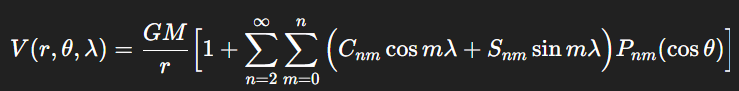
The coefficients Cnm, Snm describe irregularities in Earth’s mass distribution.
Convergence of the Series
The spherical harmonic series converges outside the smallest sphere enclosing Earth.
Inside, the series diverges.
Practically, it works for Earth’s surface and space above
R is the maximum radius of Earth and r is the distance to the evaluation point
Convergence rule: The series converges only if r > R.
Why? Because the series expansion is valid only when the evaluation point is outside the sphere containing all the mass.
If r < R, you’re inside the mass distribution, and the series diverges.
(R/r)^n —> as r increases, the ratio becomes smaller
That’s why the spherical harmonic expansion is extremely efficient for satellites in high orbits (fast convergence), but less efficient very close to Earth’s surface (slow convergence).
The harmonic expansion assumes that the mass is confined inside a sphere of radius R.
If Earth’s shape is irregular (mountains, ocean trenches, density variations), then the “effective outer radius” of the mass distribution may be larger than the chosen reference R.
If you choose R too small, some mass lies outside the assumed boundary, and the expansion becomes invalid → divergence.
Products of Inertia
They measure how mass is “spread” relative to two different coordinate planes
If the coordinate system is aligned with Earth’s principal axes of inertia (axes about which Earth naturally rotates), then the products of inertia vanish because the mass distribution is symmetric.
Forbidden or inadmissible harmonics
The spherical harmonic expansion should only include physically possible terms
Certain harmonics must vanish if the coordinate system is correctly chosen:
All degree 1 harmonics vanish —> ensures the origin is at Earth’s center of mass
Degree 2, order 1 terms vanish —> ensures the axes are aligned with Earth’s principal axes of inertia
These are called forbidden or inadmissible harmonics, because they don’t physically appear in Earth’s potential if the reference system is correct.
Normal Gravity and Level Ellipsoid
Earth is approximated by a reference ellipsoid: a smooth, rotational ellipsoid that is an equipotential surface of a normal gravity field.
The potential of this “normal field” depends only on:
Shape of ellipsoid of revolution (semi-axes a and b),
Total mass M,
Angular velocity ω
Clairaut’s Theorem
Fundamental result in geodesy that describes how gravity varies with latitude on a rotating, oblate Earth
Gravity is weaker at the equator and stronger at the poles
Cause: Earth’s rotation (centrifugal force reduces effective gravity at equator) + flattening (mass is closer to poles than equator)
Normal vertical gradient
The rate of change of normal gravity with height above the ellipsoid
Important in geodesy for reducing gravity measurements to the ellipsoid
Mean Curvature of the Level Ellipsoid
The level ellipsoid (reference ellipsoid) is not a perfect sphere but an oblate ellipsoid
Its curvature varies with latitude:
Larger curvature at the poles
Smaller curvature at the equator
Combines the principal curvatures in the meridian and prime-vertical directions
It shows how the ellipsoid “bends” as a surface of reference
Gravity Above Ellipsoid
Geoid models require all gravity values to be reduced to the same reference surface (the ellipsoid). Without this correction, you’d be mixing values taken at different heights.
Satellites orbit hundreds of km above Earth, so their measured accelerations must be “brought down” to ellipsoid height for consistency.
Gravity Anomalies Outside the Earth
On Earth’s surface, anomalies reflect density variations (mountains, ocean trenches, mantle irregularities)
Outside the Earth, anomalies are still meaningful because the disturbing potential T expands into space
Gravity anomalies at altitude can be reduced (“downward continued”) to the surface using potential theory
This allows satellites to provide global gravity anomaly data
Gravity anomalies represent mass irregularities, whether measured on Earth or above it. They’re the raw data for geoid determination.
Disturbing Potential and Anomalies
Actual potential W = normal potential U + disturbing potential T:
W = U + T
Disturbing potential T: represents irregularities caused by mountains, ocean trenches, etc.
Related quantities:
Gravity anomaly (Δg): difference between actual and normal gravity magnitudes.
Deflection of the vertical (ξ, η): angular difference between true plumb line and ellipsoid normal.
Geoid undulation (N): height difference between ellipsoid and geoid.
Fundamental Equations of Physical Geodesy
Brun’s Formula: N = T / γ
Shows that geoid height N is proportional to disturbing potential T
Δg and T are related by Poisson’s integral
Stokes’ Formula (Geoid from Gravity Anomalies)
Stokes showed that surface gravity anomalies can be integrated to compute geoid undulations:
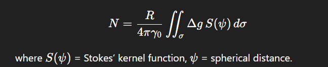
Practically:
Divide Earth into small surface elements (grids or templates)
Integrate anomalies to get N
This is the core tool for geoid determination in geodesy
It transforms local gravity anomalies into geoid height
Ellipsoidal Stokes’ function
A more precise version that accounts for Earth’s flattening. Its expression is more complex and harder to compute, so in practice most geoid models use the spherical approximation with small corrections
Methods of evaluation: templates vs. grid lines
Template Method
The Earth’s surface around the computation point is divided into small spherical trapezoids (templates)
Each trapezoid’s anomaly value is weighted with Stokes’ function and integrated
Advantage: simple concept, handles irregular distribution of data
Disadvantage: less efficient if data is on regular grids, needs careful weighting near poles
Grid-line Method
Assumes anomalies are available on a regular latitude-longitude grid
This integral is computed along grid lines of latitude and longitude, summing contributions systematically
Advantage: efficient when using global datasets (like satellite gravity grids)
Disadvantage: requires anomalies on uniform grids (interpolation may be needed)
Effect of the neighborhood
Nearby anomalies to the computation point have a much stronger influence on the computed geoid undulation than distant anomalies
Implications:
The quality of geoid determination depends critically on accurate local gravity data
Satellite data provide long-wavelength (global) accuracy, but without dense terrestrial data in the neighborhood, the geoid will be unreliable
Hence, combination models are used: satellites for large-scale features, ground data for local details