ECON 101
Day 1: Demand = Marginal Value
Postulates of Human Behavior
set of ideas about human behavior derived from observation.
People have preferences:
Given a choice between goods, consumers can make a decision about which is preferred.
Preferences can and do differ across individuals
Allows for trades to occur → willing to make tradeoffs,
not all goods are valued the same because of these preferences.
More is preferred to less
refers to all goods, not individual goods
as you have more of a good, you will want it less.
People are willing to substitute one good for another
willing to make trade-offs
The more we have of good, the less we value an additional unit of that good.
Demand Topics:
The Demand Curve
Value, Expenditure, and Net Benefits to Consumers
The decision to buy or not to buy
From individuals to markets
Quantity Demanded Vs. Demand
Shifting the Demand Curve
The Demand Curve:
The Demand Schedule:
Table showing how much of a good or service consumers will want to buy at different prices
Shows the quantity demanded of a good at various prices, holding all other factors constant, allowing for an analysis of consumer behavior in response to price changes.
The Demand Curve:
A curve that graphically represents the quantity of a particular good a consumer is willing to buy at each price level.
Summarizes the relationship between the quantity demanded of a good and the price of that good, holding all other factors constant.
Graphical representation of the SAME INFO as the Demand Schedule.
Characteristics of Curve:
Negative slope
ex: gas → don’t have to buy full unit.
ex: formulation → weekly average (incremental units)
Price = y-axis, quantity = x-axis.
Demand curves are not usually straight IRL, but easier to work with.
The Law of Demand:
The quantity demanded of a good is inversely related to the price of that good, HOLDING OTHER FACTORS CONSTANT.
As the price goes up, QD goes down
As the price goes down, QD goes up
Demand Curves are downward sloping
The more you have of a good, the less you are willing to pay to obtain another unit of that good. Holding all else constant.
Additional Concepts:
Law of Diminishing Marginal Value: As consumption of a good increases, the additional satisfaction (or utility) gained from consuming each additional unit decreases, leading consumers to value subsequent units less.
The Marginal Value of a good decreases as more units are consumed. (holding everything else constant)
reason why the Demand curve is downward sloping → because wanting less of a good.
First, good satisfied want → additional goods not needed to satisfy.
Total Expenditure (TE): The total amount of money spent by consumers on a good, calculated by multiplying the price of the good by the quantity purchased, and is influenced by changes in demand and prices.
The total amount actually spent to purchase a given quantity of a good.
TE= PxQ, where TE represents Total Expenditure, P denotes the price per unit of the good, and Q refers to the quantity purchased.
Consumer Surplus (CS): The difference between what consumers are willing to pay for a good or service and what they actually pay; it represents the benefits to consumers from participating in the market. Consumers experience surplus when the market price is lower than their maximum willingness to pay, and can be calculated graphically as the area between the demand curve and the market price level.
Net benefit to consumers
The difference between what a consumer would be willing to pay for the units purchased (TV) and what the consumer actually pays (TE).
CS= TV-TE → willing-actual
Consumers want the highest CS possible.
How Many Units will an individual consume?
Consumption decision depends upon:
Price: how much a consumer must give up for each additional unit
Assume the same price for all units consumed
Marginal Value: how much the consumer is WILLING to give up for each additional unit consumed
recall DMV
Will continue to consume as long as the MV for an additional unit is greater than or equal to the Price
Stop consuming the good at the point where MV=Price (benefits equal cost)
Do not consume where MV<Price (cost exceeds benefits)
Day 2: Market Demand
Interpretations of market demand curve similar to individual demand curves. → sum of all CS
The height of the demand curve at a given quantity represents the Marginal Value (MV) of the good at that quantity
Area under the demand curve up to the quantity consumed equals the Total Value (TV) for all consumers in the market.
The area between the demand curve and price is the Consumer Surplus (CS) gained for all consumers in the market.
Law of Demand: As price falls, quantity demanded increases → inverse relationship
Those currently consuming the good consume more.
New consumers enter the market
Quantity Demanded vs. Demand:
Quantity demanded: The actual amount of a good that consumers are willing to buy at some specific price.
A point on a demand curve at a specific price.
Change in QD is a movement from ONE POINT on the demand curve to another point on the demand curve.
A movement along the same demand curve in response to a change in price. (holding all else constant)
A movement from a point on one demand curve to a point on another demand curve in response to a change in some factor other than price.
Demand: Shows the amount of a good consumers are willing to buy at every price.
The entire demand curve
A Change in demand is a shift in the entire curve.
Shifts of the Demand Curve:
An “increase in demand” means a rightward shift of the demand curve: at any given price, consumers demand a larger quantity than before.
Other Factors that cause the entire demand curve to shift:
A change in the price of related goods:
Complements: consumer goods
Two goods used jointly in consumption → iPad and Apple Pencil
If the price goes up for one QD, changes → at every price, people buy less.
An increase in the price of a complement results in a leftward shift in the demand curve.
A decrease in prive of a complement results in a rightward shift in the demand curve
Substitutes:
Two goods that satisfy similar wants or desires
An increase in the price of a substitute results in a rightward shift in the demand curve
A decrease in the price of a substitute results in a leftward shift in the demand curve.
Changes in income:
Normal goods:
A good for which demand increases when income increases
An increase in income causes a rightward shift in the demand curve
A decrease in income causes a leftward shift in the demand curve
Inferior goods:
A good for which demand decreases when income increases
An increase in income causes a leftward shift in the demand curve
A decrease in income causes a rightward shift in the demand curve
No good is inferior to everyone.
Change in the number of consumers:
An increase in the number of consumers leads to a rightward shift in the demand curve
A decrease in the number of consumers leads to a leftward shift in the demand curve.
Change in information about the Uses of a Good:
Depends on the type of information
Change in expectations about Future Prices:
If you expect the future price to be higher, it leads to a rightward shift in the demand curve today
If you expect the future price to be lower, it leads to a leftward shift in the demand curve today.
Have to be able to store it, though.
Day 3: Supply = Marginal Cost
The Supply Schedule:
The table shows how much of a good or service suppliers will want to sell at different prices, holding all other factors constant.
Their willingness to sell it
The Supply Curve: UPWARD SLOPING
A curve that graphically represents the quantity of a particular good a supplier is willing to sell at each price level.
Summarizes the relationship between the quantity supplied of a good and the price of that good, HOLDING ALL OTHER FACTORS CONSTANT.
Graphical representation of the supply schedule
The quantity supplied of a good is typically positively related to the price of that good, holding other factors constant.
As the price goes up, the quantity supplied goes down
As the price goes down, quantity supplied goes down
Ex: oranges in Florida → as the price of oranges increases due to higher demand, farmers are incentivized to supply more oranges to the market.
Total Cost (TC): Cost of all units of output currently produced.
Inputs need to be used; all of these have alternatives.
TC= MC + fixed cost
fixed cost: factory → upfront cost to do anything could be different things.
Sum of marignal costs for all units produced=variable cost.
Marginal Cost (MC): Cost of producing an additional unit of output
cost of production → TC=everyone, MC=One
Total Revenue (TR): The sum of receipts a firm receives from the sale of output → sum of the sales.
PxQ sold (usually equal to Total Expenditure)
Producer Surplus (PS): The difference between the price sellers receive for a good and the marginal cost of producing the good.
Net benefits to the supplier.
How Much Will The Producer Supply?
Supply decision depends upon:
Price: how much the supplier receives for each unit produced → want the highest price
Assume the same price for all units produced.
The marginal cost of producing an additional unit of a good.
Will continue to supply as long as Price recieved for an additional unit is greater than or equal to the Marginal Cost of producing that unit.
Stop producing the good at the point where MC=P
If MC=P, assume it will produce a unit
Do not produce if MC>P (costs exceeds benefit)
Individual supply curve and the market supply curve: The Market supply curve is the horizontal sum of the individual supply curves of all firms in that market.
Quantity Supplied Vs. Supply:
Quantity supplied: the actual amount of a good that suppliers are willing to sell at some specific price
A point on the supply curve at a specific price.
Change in QS is a movement along the supply curve, reflecting how the quantity supplied varies in response to price changes.
A movement along the same supply curve in response to a change in price (holding all else constant)
Supply: shows the amount of a good that suppliers are willing to sell at every price.
The entire supply curve
A change in supply is a shift in the entire supply curve.
Factors that cause the entire supply curve to shift: Any “decrease in supply”=left, increase is to the right
Change in the price of inputs:
Land, Labor, and capital
resources are used in the production of the good.
An increase in the price of an input results in a leftward shift
decrease in the price of an input results in a rightward shift
Changes in technology:
Changes the cost of production
If technological change reduces the cost of production, the result is a rightward shift
If technology increases the cost, then the leftward shift
Change in the number of suppliers:
An increase in the number leads to a rightward shift
A decrease is a leftward shift
Change in expectations about future prices:
If you expect future prices to rise, it leads to a leftward shift in the supply curve today
If you expect the price to be lower, it leads to a rightward shift in the supply curve.
Day 4: Equilibrium
Benefits of exchange:
Voluntary exchange is based on mutual benefits.
If we agree to trade, then both parties must perceive net benefits, or else they would not engage in voluntary trade.
Net Benefits:
Consumer: CS
Supplier: PS
Gains from trade:
Demand Curve (Consumers)
Recall, the height of the demand curve at a given quantity represents consumers’ marginal willingness to pay for that last unit (MV)
Supply Curve (Producers)
Recall, the height of the supply curve at a given quantity represents the producer’s marginal cost to produce that last unit (MC)
If the MV to consumers exceeds the MC to producers for a particular unit, then there exists potential gains from trade for both parties
Beneficial trade continues until MV=MC → equilibrium
All gains from trade are exhausted (have been realized)
Economic efficiency: total benefits at maximum → when MV=MC
All mutual benefits from trade are exhausted.
Net benefits to society are maximized
Efficiency doesn’t imply equity, and may not be desirable
Market Clearing Price: Price at which QD=QS
All consumers are willing to buy at this price
All suppliers willing to sell at this price can find a buyer.
Price is higher than the market cleaning price:
Suppose the price that exists in the market is 4 per unit (higher than the equilibrium price of 3)
At this price, suppliers are willing to supply 40 units
At this price, consumers are willing to buy 20 units
There exists an excess of supply (surplus) equal to 20 units
Sellers intedned to sell these 20 units at a 4 price, but are unable to find buyers at this price.
In order to rid themselves of these excess, unwanted inventories, Sellers will begin to lower prices until the market-clearing price is reached.
Price Lower than market-clearing price:
Suppose the price that exists in the market is 2 (equilibrium is 3)
At this price, the suppliers are willing to supply 20
Consumers are willing to buy 40
There exists excess demand (shortage) equal to 20 units.
Suppliers find they cannot keep items in stock and can charge a higher price
Some consumers value this good more highly than others, paying higher prices
Price of the good gets “bid” up to the market-clearing price.
Market Equilibrium occurs where the supply curve and the demand curve intersect.
Shocking the System: Once at market-clearing price, no reason to expect the market price to change
Sellers would like to change to a higher price, but would end up with excess supply
Consumers would like to pay a lower price, but not everyone who wants the good at that lower price would be able to buy it, excess demand.
Unless something causes the demand curve or supply curve to shift.
Changes in demand:
Increase in demand:
Rightward shift in the entire demand curve
movements along the same supply curve
change in QS due to change in price
Impact on market equilibrium:
Equilibrium price rises, equilibrium quantity rises.
Decrease in Demand:
Leftward shift in the entire demand curve
Movement along the same supply curve
Impact on market equilibrium:
Equilibrium price falls, equilibrium quantity falls.
Ex: An increase in demand will lead to higher prices and quantity as a movement along the supply curve will lead to a higher equilibrium.
Change in Supply:
Increase in supply:
Rightward shift in the entire supply curve
movement along the same demand curve
change in QD due to change in prices
Impact on market equilibrium:
Equilibrium price falls, equilibrium quantity rises.
Decrease in Supply:
Leftward shift in the entire supply curve
movement along the same demand curve
Impact on market equilibrium:
Equilibrium price rises, equilibrium quantity falls.
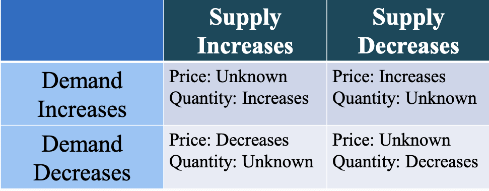
Simultaneous shifts of supply and demand curves:
Day 5: Elasticity part A
Types of Elasticity: A measure of the responsiveness of one variable to changes in another variable
4 main types:
Price Elasticity of Demand: The measure of responsiveness of quantity demanded to changes in price.
movement up or down the curve
Income Elasticity of Demand: The measure of the responsiveness of quantity demanded to changes in income.
Cross Price Elasticity of Demand: Measure responsiveness of quantity demanded to changes in the price of related goods
Price Elasticity of Supply: The measure of responsiveness of quantity supplied to changes in price
movement up or down the supply curve
Changes in QD in response to changes in price: an increase in the price of a substitute good often leads to an increase in quantity demanded of the original good, while an increase in the price of a complement can lead to a decrease in quantity demanded.
Price and QD are inversely related:
Law of Demand → useful to know in this case, but provides no information on the magnitude of changes.
How Responsive is a good?
Firms: If they increase the price, QD falls
How much + What will happen to total revenue?
This depends on the price elasticity of demand; if demand is elastic, total revenue will decrease, whereas if demand is inelastic, total revenue may increase.
Tax implications: If you raise tax on an item, the price will rise, and quantity will fall.
What will happen to total tax revenue?
The effect on total tax revenue will depend on the elasticity of demand; if demand is inelastic, total tax revenue may increase despite the decrease in quantity sold, whereas if demand is elastic, total tax revenue could decrease as the higher price leads to a significant drop in quantity demanded.
Who ends up paying the tax?
Some firms eat some of it, so demand doesn’t drop.
Price Elasticity of Demand: A measure of the responsiveness of QD to changes in price.
Provides information on how much QD will change in response to a price change
Look at percentage changes, not absolute changes
PED: % change in QD/ % change in price=-x/1
Calculating using the Midpoint Method: This method allows us to find a more accurate measure of price elasticity of demand (PED) by calculating the percentage change in quantity demanded (QD) and price based on the average of the starting and ending values. The formula to apply is:
PED= Q2-Q1/Q2+Q1/2 // P2-P1/P1+P2/2
Ratio of the percentage change in QD to the percentage change in price as the move along the demand curve.
Must be a negative number because downward sloping and the LAW OF DEMAND
Unit-free measure because all units cancel
Interpreting Price Elasticity of Demand:
PED: % change in QD/ % change in price=-x/1
If the price goes up 1%, then QD will fall by x%
If the price goes down by 1,% then QD will rise by x%
Range of values:
Elastic Demand: -infinity < E < -1, indicating that consumers are highly responsive to price changes.
Demand will change significantly because QD is very responsive to changes in price.
Unit Elastic Demand: E = -1, meaning that the percentage change in quantity demanded is equal to the percentage change in price, resulting in no overall impact on total revenue.
Inelastic Demand: -1 < E < 0, which indicates that consumers are less responsive to price changes, leading to a relatively stable quantity demanded despite fluctuations in price.
won’t lose many customers if we change the price.
Elasticity and “steep” demand curves: STEEPER MORE INELASTIC
Retaively steep demand curves: Relatively large price changes associated with small quantity changes
QD is relatively less repsonsive ot changes in price → INELASTIC
Perfectly Vertical Demand curves: QD is totally unresponsive to changes in price → perfectly INELASTIC
ex: Insulin
Elasticity and Flat demand curves: FLATTER MORE
Relatively flat demand curves: relatively small price changes associated with large quantity changes.
QD is relatively more responsive to changes in price → ELASTIC
Perfectly horizontal demand curves:
QD is completely responsive to changes in price → ELASTIC
Determinants of Price Elasticity of Demand:
Available substitutes:
More substitutes mean more opportunity to alter behavior in response to price changes.
MORE SUBS=MORE ELASTIC
Time:
The more time that passes since the price change means more opportunity to adjust behavior in response to price changes.
How Narrowly Defined:
More narrowly defined means more substitutes → MORE ELASTIC
ex: Food (inelastic), apples (elastic)
Day 6: Elasticity part B
Changes in Elasticity along a linear demand curve:
Just to complicate things, Price elasticity of demand will change depending on the current price and quantity.
Even along a linear demand curve (straight line demand curve with a constant slope)
Elasticty of demand doesn’t equal slope of demand curve; instead, it is a measure of the responsiveness of quantity demanded to a change in price, which varies at different points along the curve.
Unit-Elastic, inelastic, or Elastic?
The classification between them predicts how changes in the price of a good will affect the total revenue earned by producers from the sale of that good.
The total revenue is defined as the total value of sales of a good or service
Total revenue= Price x Quantity Sold. Therefore, when demand is elastic, a decrease in price will lead to an increase in total revenue, while an increase in price will decrease total revenue. Conversely, if demand is inelastic, changes in price will have a lesser effect on total revenue.
When a seller raises the prices of a good, there are two countervailing effects in action (except in the rare case of a good with perfectly elastic or perfectly inelastic demand)
A price effect: After a price increase, each unit sold sells at a higher price, which tends to raise revenue.
Making more off people who are still buying it
A quantity effect: After a price increase, fewer units are sold, which tends to lower revenue.
Losing quantity sold.
If demand for a good is elastic (the price elasticity of demand is less than -1)
In this case, the unitary effect is stronger than the price effect
An increase in the price reduces total revenue
If demand for a good is inelastic (the price elasticity of demand is between 0 and -1)
In this case, the price effect is stronger than the quantity effect
An increase in price increases total revenue.
Ex: gas or coffee
If demand for a good is unit-elastic (the price elasticity of demand is exactly -1)
In this case, the quantity effect and the price effect exactly offset each other
An increase in price doesn’t change total revenue.
Other types of elasticity:
Income elasticity of demand: the percent change in the quantity of a good demanded when a consumer’s income changes, divided by the percent change in the consumer’s income
IED=% change in QD/% change in income
When the income elasticity of demand is positive, the good is a normal good, that is, the quantity demanded at any given price increases as income increases.
If positive and greater than 1, then it is considered income elastic
If positive and less than 1, then considered income elastic
When the income elasticity of demand is negative, the good is an inferior good, that is,s the quantity demanded at any given price decreases as income increases.
Cross price elasticity of demand: between two goods measures the effect of the change in one good’s price on the quantity demanded of the other good.
It is equal to the percent change in the quantity demanded of one good divided by the percent change in the other good’s price.
The CPE between good A and B = % change in quantity demanded of good A ÷ % change in price of good B.
A positive CPE indicates that the two goods are substitutes, while a negative CPE suggests they are complements.
Price elasticity of supply: a measure of the responsiveness of the quantity of a good supplied to the price of that good.
It is the ratio of the percent change in the quantity supplied to the percent change in the price as we move along the supply curve
Ranges are the same as the price elasticity of demand
PES= % change in quantity supplied / % change in price
Determining factors:
The availability of inputs: the price elasticity of supply tends to be large when inputs are readily available and can be shifted into and out of production at a relatively low cost. Tends to be small when inputs are difficult to obtain
Time: The price elasticity of supply tends to grow larger as producers have more time to respond to a price change. This means that the long-run price elasticity of supply is often higher than the short-run elasticity.
There is a perfectly inelastic supply when the price elasticity of supply is 0, so that the change in the price of the good has no effect on the quantity supplied. A perfectly inelastic supply curve is a vertical line
There is a perfectly elastic supply when even a tiny increase or reduction in the price will lead to very large changes in the quantity supplied, so that the price elasticity of supply is infinite. A perfectly elastic supply curve is a horizontal line.
Day 7: Price Controls
Review of Key Concepts:
Market Clearing Price: Price at which QD=QS
If the market price is not the market-clearing price, neither demanders nor suppliers have incentives to alter their behavior to drive the price back to the market-clearing price
Economic efficiency: All mutual benefits from trade are exhausted
Net benefits to society are maximized.
Deadweight Loss: Lost benefits to society that occur whenever output differs from the efficient quantity
Monopolies, price controls, taxes, and oligopoly
Price Control: Legal restriction on how high or low a market price may go
Enacted by governments
Price Ceiling: A maximum price sellers are allowed to charge for a good
Only binding if below market clearing price
Ex: rent controls, electricity prices, gas prices (1973-74)
Outcomes:
Persistant shortage
Redistribution of economic welfare → Every policy has its
Winners: Consumers are able to buy the good.
Losers: Suppliers and consumers unable to buy the good (excess demand)
Non-price rationing: Some rationing mechanism must determine who among the 400 demanders receives the 200 units supplied at the price ceiling.
Normally price would rise to ration, but not allowed to do so in this case.
Ex: Waiting in line (Time cost), Favoritism/discrimination (illegal but still occurs), Violence, lottery, lobbying, black market.
Graphical analysis provides “Best Case Scenario”: Conditional on a shortage occurring, the graphical analysis provides the largest possible consumer surplus and the minimum possible deadweight loss.
Inefficient Allocation: In most cases, there is no guarantee that those who value the good the most are able to acquire the good.
Would further reduce the consumer surplus
Wasted Resources: Some form of rationing mechanism will determine who receives the good (non-price rationing)
Additional costs are likely to be incurred.
Ineffceiently Low Quality:
Some consumers are willing to pay more in order to receive higher quality.
Suppliers are unable to raise the price (illegal to do so)
Exists little incentive for suppliers to increase or maintain quality.
Price floor: Aminimum pirce buyers are required to pay for a good.
Only binding if above market clearing price
A minimum price that demanders must pay for the good
Examples: Agricultural price supports, minimum wage, alcohol, and cigarettes.
Minimum wage: The lowest hourly wage that employers can legally pay their workers, aimed at ensuring a basic standard of living for employees.
Little empirical evidence for the unemployment effect
Firms could raise prices, cut down on working hours
Wage compression, lower profits, reduction in hirings, trainings, and benefits.
Offsetting benefits: paying people more could increases prodcutivity
lower turnover rates, which saves firms money
Other effects: some firms don’t pay it anyway, even though it’s illegal (the largest theft inthe country is wage theft).