Week 12: Mixed Factorial ANOVA
Introduction
Mixed-factorial ANOVAs are used to test data from factorial research designs.
Factorial designs involve more than one IV.
Mixed-factorial ANOVAs include a mix of between-groups and repeated-measures IVs.
Overview of Mixed Factorial ANOVA
Mixed Factorial ANOVA: A statistical test used to examine the effects of two or more IVs on a DV, where at least one IV is a between-groups factor and at least one is a repeated measures factor.
Between-Groups IV: Different groups of participants are exposed to different levels of this factor; each participant experiences only one level of this IV.
Example: Randomly allocating one group of participants to CBT and another to general counseling.
Repeated Measures IV: All participants are exposed to all levels of the factor.
Example: Measuring all participants at three time points: baseline, after two weeks, and after six weeks.
Mixed Factorial ANOVA combines both between-groups and repeated-measures IVs.
Example: Randomly allocating participants to CBT or general counseling (between-groups IV) and measuring anxiety symptoms at baseline (Time 1), after 2 weeks (Time 2), and after 6 weeks (Time 3).
Mixed Factorial ANOVA tests both the main effect of IVs and the interaction between them.
Benefits of mixed factorial research:
Allows measurement of the effect of a between-groups IV to see if there are differences between groups.
Tests if different groups change in the same way across repeated-measures conditions.
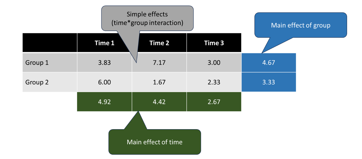
Main Effects and Interactions in Mixed Factorial ANOVA
Main Effects:
Between-groups IV: Indicates whether there is a significant difference in mean scores between the groups, ignoring the repeated-measures IV.
Repeated measures IV: Indicates whether there is a significant difference in mean scores between repeated measures conditions, ignoring the between-groups IV.
Interaction Effect:
Indicates if the effect of one of the IVs is different at different levels of the other IV.
Two ways to think about the interaction:
Does the effect of the repeated measures IV differ at different levels of the between-groups IV?
Does the DV change across repeated measures conditions?
Is the pattern of change over time the same for each group?

Does the effect of the between-groups IV differ at different levels of the repeated measures IV?
Are there differences between groups?
Are these differences the same at each time point?

When Would You Use a Mixed Factorial ANOVA?
Whether a repeated-measures intervention leads to different results for different groups.
Example: Significant reduction in anxiety symptoms after 3 weeks and 6 weeks of CBT, compared to baseline, and is the degree of change the same for participants with and without GAD?
Design: 3 (time point: baseline, 3 weeks, 6 weeks) x 2 (Group: GAD, no GAD).
Does a DV change across time in the same way for people in different experimental conditions?
Example: Do anxiety symptoms change between baseline and a 2-week follow-up test for people in a control group and for people receiving CBT?
Design: 2 (time point: baseline, 2 weeks) x 2 (Treatment: Control, CBT).
Types of Data Suitable:
DV must be continuous.
At least one between-groups IV that is categorical.
At least one repeated-measures IV that includes two or more time points.
Assumptions of Mixed Factorial ANOVA
Normality of Residuals:
Factorial models assume that the residuals of the model are normally distributed.
Evaluated using a normal Q-Q plot.
ANOVA is robust to violations of normality, particularly when sample sizes are large.
Severe departures from normality can affect the validity of ANOVA results.
Can consider transforming variables or using an alternative statistical test.
Homogeneity of Variance:
The variances of the different groups are approximately equal.
For mixed-factorial designs, check this at each level of the repeated-measures variable.
Levene's test is used to assess homogeneity of variance.
If p < .05, the assumption of homogeneity is violated.
If p > .05, the assumption of homogeneity is satisfied.
Sphericity:
The variability in differences between time-points is equal.
Mauchly's test is used to test the assumption of sphericity.
If p < .05, the assumption of sphericity is violated.
If p > .05, the assumption of sphericity is satisfied.
Corrections for Violation of Sphericity:
Apply a Greenhouse-Geisser or Huynh-Feldt correction.
If Ɛ < .75, choose the Greenhouse-Geisser correction.
If Ɛ > .75, use the Huynh-Feldt correction.
The assumption of sphericity is always met if your repeated measures IV only have two levels.
Interpreting the output and reporting the results
Omnibus Tests
Degrees of freedom (df): Represents the amount of information that can freely vary.
F statistic: The omnibus test for each effect.
Effect size: Partial eta squared (\eta_p^2), which tells us how much variance in the DV the effect accounts for.
Within-Subjects Effects table
Provides results for the main effect of the repeated-measures IV and the interaction between the between-groups and repeated measures IVs.
Example: Main effect of time is significant and accounts for 49% of variance in satisfaction ratings, F(2, 20) = 9.67, p = .001, \etap^2 = .49. The interaction between time and participant group is significant and accounts for 72% of variance, F(2, 20) = 26.26, p < .001, \etap^2 = .72.
Between-Subjects Effects table
Provides results for the main effect of the between-groups IV.
Example: The main effect of group is significant and accounts for 38% of variance in satisfaction ratings, F(1, 10) = 6.15, p = .033, \eta_p^2 = .38.
Simple Effects (Post Hoc Tests)
Pairwise comparisons to understand the interaction effects, often using t-tests.
Tukey correction may be used to adjust for inflated Type 1 errors.
Report t-test results as: t(df) = X.XX, p = .XXX.
Descriptive statistics (Ms, SDs) should be reported to provide a sense of the magnitude of each difference.
Simple Effects Plot
Provides a visual illustration of the simple effects.
Example Summary:
Customers: Satisfaction levels increase from Time 1 to Time 2, then decrease at Time 3.
Employees: Satisfaction levels decrease from Time 1 to Time 2, and then remain low at Time 3.
Descriptive Statistics
Report means and standard deviations for each group at each level of the repeated measures IV.
General guidelines for reporting results of a mixed factorial ANOVA
Report the results of the omnibus tests for both the main effects and interaction: F(df1, df2) = X.XX, p = .XXX
If the interaction is significant, report the simple effects and specify if a correction was applied to them.
Report each of the key comparisons that relate to your hypotheses.
Include descriptive statistics (M, SD) for each group, if they are significantly different or not and the direction of the difference.
E.g., At Time 1, Group 1 (M = X.XX, SD = X.XX) had significantly higher scores than Group 2 (M = X.XX, SD = X.XX), t(X) = X.XX, p =.XXX.
If the interaction is not significant, do not run simple effects. Instead, report the results of post-hoc comparisons for each main effect (describe if any corrections were made, provide descriptive stats, t-test results, and effect size for each post-hoc comparison).