Marginal rate and substitution

• MRSxy = oppurtunity cost, slope of indifference curve

A series of optimal consumer choices provides the theoretical basis for an individual demand curve

Diminishing marginal utility

• as we consume more of a good, the satisfaction we derive from 1 additional unit decreases

• rate of satisfaction diminishes with every 1 unit

• examples: food, cars

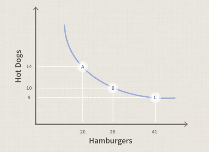
Indifference curves

• IC always has a negative slope if consumer likes both goods

• IC cannot intersect

• Every good can lie on one IC

• ICs are not thick

Demand Theory

• Substitute effect

  • Measures of consumer MRSxy, before and after the price change

  • Amount of additional food the consumer would buy to achieve the same level of utility (assuming a price decrease in one good)

  • Moving from one optimal curve to another

  • Steps:

    • Identify initial optimum basket of goods

    • Identify final optimum basket of goods, after the price change

    • Identify the decomposition optimum basket (DOB), attributed to the substitution effect

      • DOB must be on a BL that is parallel to BL2 following the price change

      • Assume that consumer retains same level of utility after the price change

• Income effect

  • Accounts for price change by holding the consumer’s purchasing power (following price change) constant and finding an optimum bundle on a new (higher/lower) utility function

    • Purchasing power - number of goods/services that can be purchased with a unit of currency (falls when price increases)

  • Measured from the DOB (B and Xb) to the final optimum bundle, following price change (C and Xc)

  • Both effects move in the same direction

• Law of Demand

  • At a higher price, consumers will demand a lower quantity of a good (vice versa)

  • Relates to diminishing marginal utility by compensating (off-set) DMU must be negatively related to quantity

  • Inverse relationship of price and quantity

  • Given the presence of diminishing marginal utility, in order to promote increased consumption, prices must fall

  • For a “normal good,” the increase in consumption results from a fall in price - this is driven by:

    • a lower MRSxy, while remaining on the same IC generates increased consumption of good X (substitute effect)

    • the theoretical increase in income necessary to lift the consumer to the higher IC, while keeping the ratio of prices at the new level (income effect)

  • Economic theory of demand always starts at the individual level. A horizontal summation of many individual demand curves provides a market demand curve. Market demand curves are always less steep than individual demand curves

Determinants of Demand

• Income

• Price of substitutes/complements

• Number of consumers

• Preference or tastes

  • These factors cause a market demand curve to shift (change in demand)

Individual Demand Curve

• a series of optimal choice bundles across different price levels (shown on price-quantity graphs)

Inferior Good

• whether the substitution effect or income effect dominates in an empirical not theoretical question

• Opposite of a normal good, demand falls when income rises

Non-price determinants of demand

• income (normal good)

• income (inferior good)

• preferences/tastes

• price of substitute/complement goods

• number of consumers

Perfect Competition

• Economic profit maximization is the assumed goal of private firms

  

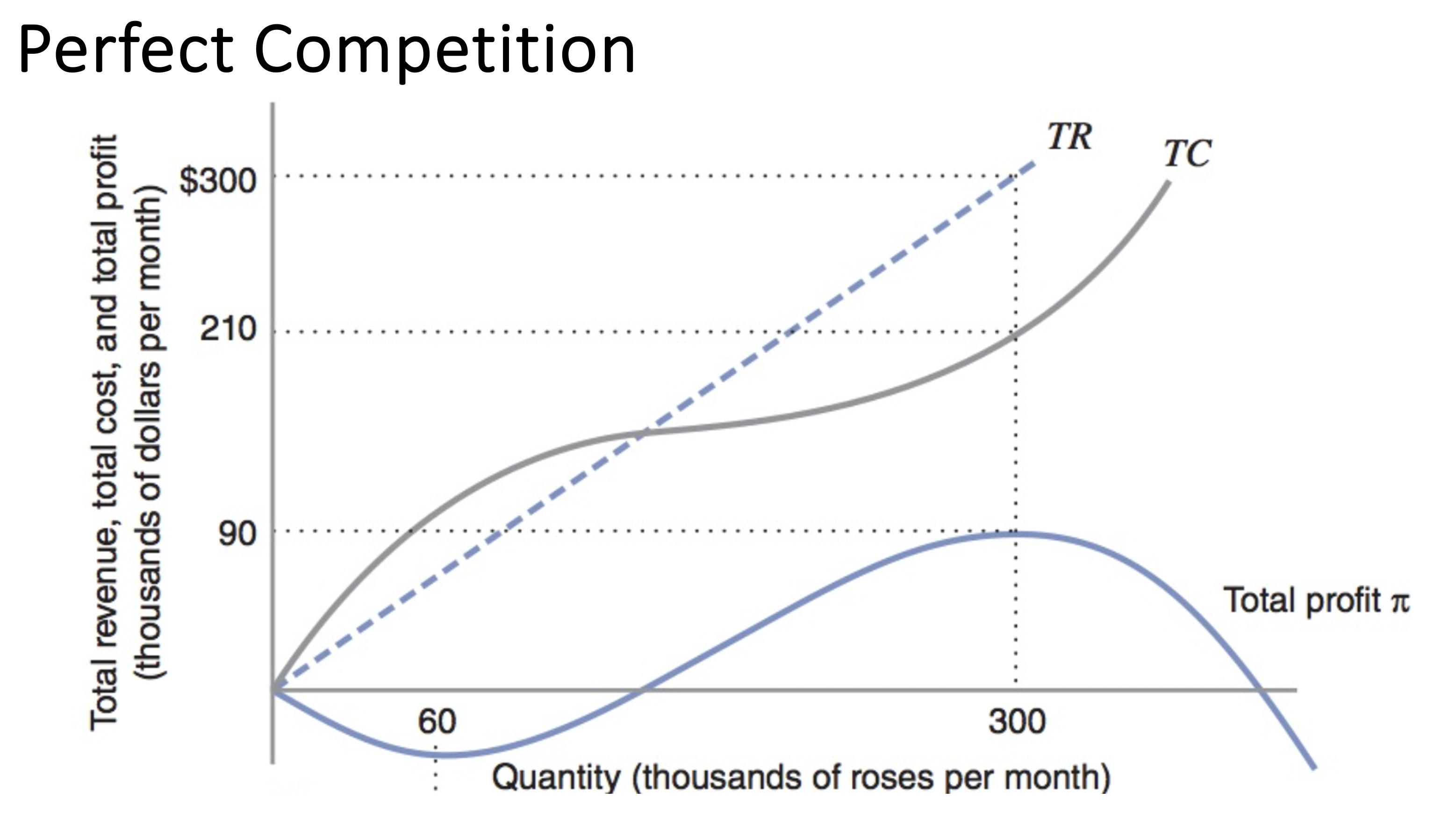
• Total cost represents the most efficient combination of inputs for a given level of output

• The rate at which total revenue (TR) changes with respect to change in output (Q) is marginal revenue (MR)

• MR = TR/Q = (Q*P)/Q = P

  

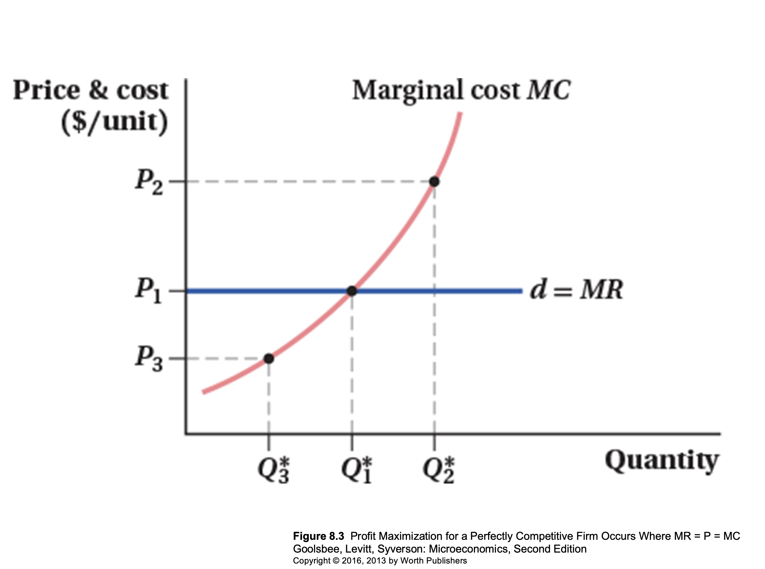
• Profits are maximized when marginal revenue = marginal cost

  • After the point where MR=MC, your profits will be negative

• Supply = MC, total cost optimized

Market Equilibrium

• the intersection of the demand and supply curves

• total cost is important as it is the basis of an individual firm’s supply curve

  • upward sloping section of the marginal cost curve is the supply curve

Efficiency of demand/supply curves

• Supply curves

  • Optimal combination of cost-minimizing inputs for each level of output

• Demand curves

  • Optimal combination of utility-maximizing goods for a given level of income

• Market supply curve

  • Horizontal summation of a series of individual supply curves

Supply Theory

• Supply - total amount of goods and services that producers are willing and able to purchase at a given price in a given time period

• Law of Supply

  • as the price of a product rises, the quantity supplied of the product will usually increase (ceteris paribus)

  • firms attempt to maximize product by increasing quantity supplied when the price is higher (and vice versa)

Non-price determinants of supply

• Changes in costs of factors of production

• Prices of related goods

• Indirect taxes and subsidies

• Future price expectations (producer)

• Changes in technology

• Number of firms

• Shocks

  • Markets only work when there is strong competition

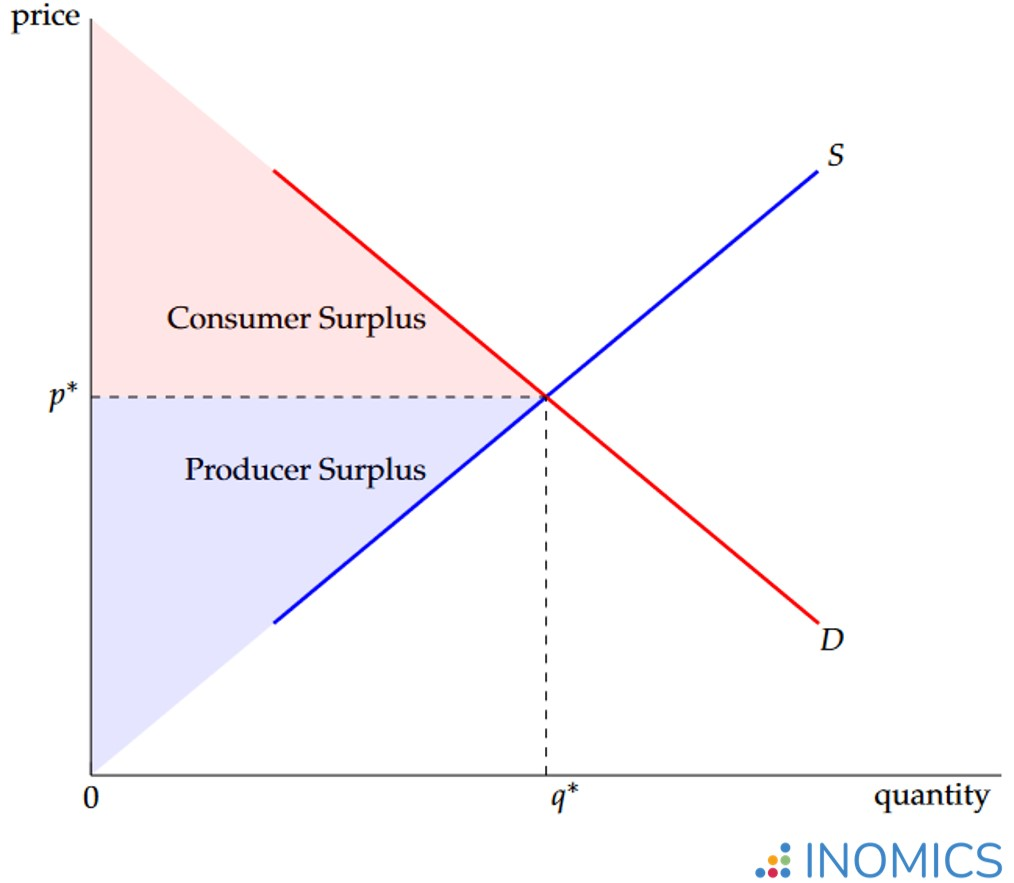
Market Equilibrium Graphs (supply + demand)

Consumer Surplus (C.S.) - willingness to pay and what they did pay

Producer Surplus (P.S.) - difference between market price and lowest price a producer uses to produce

Assumptions of perfectly competitive markets

• all actions (consumers/producers) have access and fully process all relevant information

• there are many small buyers and producers - all with equally negligible market power

• all actors are rationally self-interested

Welfare - theoretical surplus value left with different economic agents (consumers, firms, governments)

Production - market clearings

Optimal Allocation

• MR = MB (marginal benefit)

• Social surplus = consumer + producer surplus

• In a perfectly competitive market, social surplus is at its largest

• Analysis of surpluses are called “welfare analysis”

Price Mechanism Functions

A - allocation (resources are allocated to those who need it most)

R - rationing (not everyone in the market gets what they want, only those who have the same valuation of the product as the firms)

S - signaling (communication of information that drives other factors)

I - incentive (capitalist system is driven by incentives)

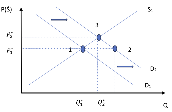
2 Demand Curves

2 Supply Curves

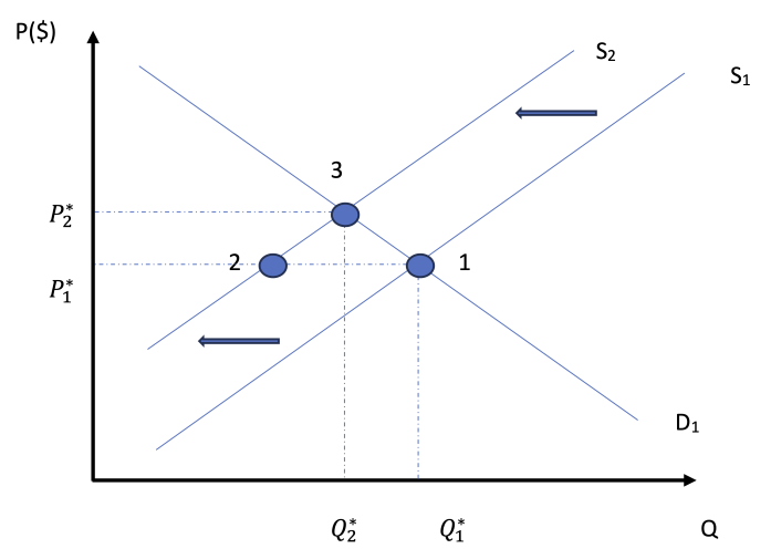
• Moving from point 1 to point 3 on both graphs

• Point 2 has excess supply/demand

• ARSI to move to the new equilibrium point

• At both equilibriums, there is optimal allocation

Structure of Microeconomics

• How do consumers and producers make choices in trying to meet their economic objectives?

  • Demand

  • Supply

  • Competitive market equilibrium

  • Elasticities of Demand

  • Elasticities of Supply

  • Critique of the maximizing behavior of consumers and producers

  • interaction between consumers and producers determine where resources are directed

  • welfare is maximized if allocative efficiency is achieved

  • constant change produces dynamic markets

  • consumer and producer choices are the outcome of complex decision making

• When are markets unable to satisfy important economic objectives - and does government interaction help?

  • Role of government in microeconomics

  • Market failure

    • externalities and common pool or common acess resources

    • public good

    • asymmetric information (imbalanced information held by consumers and/or consumers)

    • market power (single/small number of suppliers)

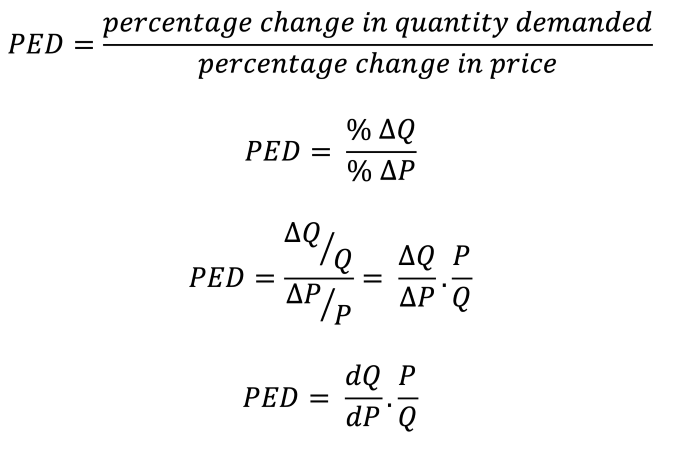
Price Elasticity of Demand (PED)

• measure of the responsiveness of the quantity demanded of a good subject to the change in price

  • Percentage change and differentiation to calculate

• PED = percentage change in quantity demanded / percentage change in price

  

• |PED| > 1 demand is relatively elastic

• |PED| < 1 demand is relatively inelastic

• |PED| = 0 demand is unitary

• PED = ∞ perfectly elastic

• PED = 0 perfectly inelastic

How can PED change along a straight line?

• as you move along the x-axis, it gets less elastic

  • as quantity increases, elasticity decreases

How does PED change across income levels?

• more elastic for lower income groups

• elasticity depends on the good (price-quantity relationship)

• quantity demanded changes, but not the demand curve

• “staples” are essential, less elastic

Determinants of Price Elasticity of Demand (PED)

• number of close substitutes; more subs = increased price sensitivity

• luxuries VS staples

• time - purchases made with longer time periods are generally more elastic

• proportion of income spent on the good

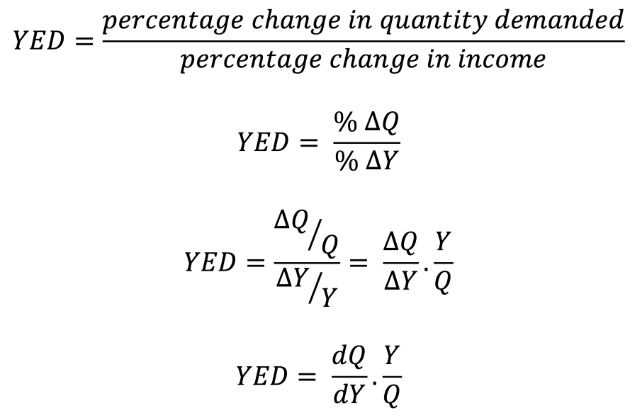
Income Elasticity of Demand (YED)

• measure of how much demand for a product changes when there is a change in the consumer’s income

• YED = percentage change in quantity demanded / percentage change in income

  

• YED to categorize inferior and normal goods

Engel Curve

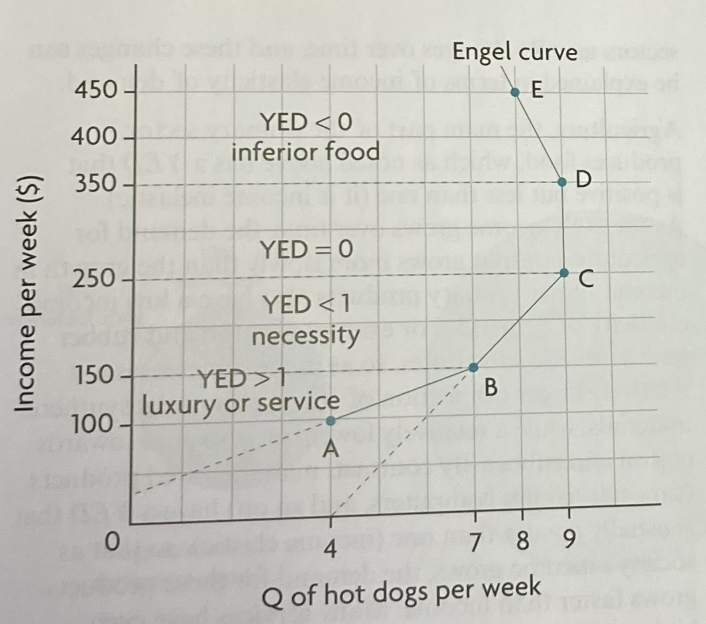
• axes → income and quantity

• YED > 1 luxury/service

• YED < 1 necessity

• YED > 0 normal good

• YED < 0 inferior good

• quantity demanded when income increases also increases then diminishes and goes backwards

• if you continue a segment AB with the same slope and that line cuts the y-axis, then it is a luxury

  • if it cuts the x-axis, it is a necessity

  • only works on income = y and quantity = x

Primary Commodities

• raw materials (cotton, coffee)

• inelastic demand (they are necessities)

• consumers are not everyday households, but manufacturers

Manufactured Goods

• made from primary commodities

• more elastic, as there are more substitutes

Why is YED important?

• For firms:

  • products with a high YED will see a demand increase when income increases (used to see maximum profit based off changes in income)

    • allocation of resources to fit income groups in products

    • if income falls, production of inferior goods increase because of YED rules

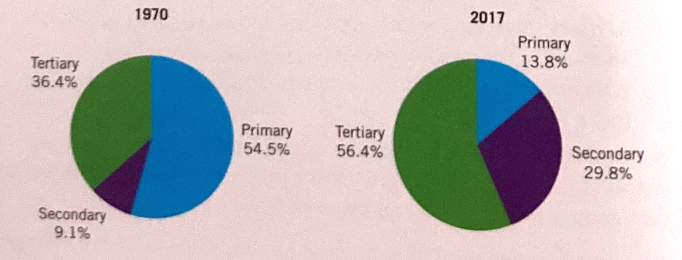
• Sectoral changes

  • primary sector: agriculture, fishing, extraction (forestry, mining)

  • secondary sector: manufacturing, takes primary products and uses them to manufacture producer goods (machinery, consumer goods) also includes construction

  • tertiary sector: service, produces services or intangible products (financial, education, information, technology)

  • shifts in the relative share of national output and employment

  • as countries grow and living standards improve, there is a change in proportion of the economy that is produced

  • extra income is spent on manufactured goods as the demand is more elastic than the primary products (using YED to measure/verify) ← same goes for the service sector

    

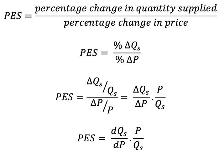
Price Elasticity of Supply (PES)

• PES = percentage change in quantity supplied / percentage change in price