AP Physics C: Mechanics - Unit 1: Kinematics
1. Fundamentals of Motion and Vectors
Definitions & Conceptual Basics
Kinematics is the branch of mechanics describing the motion of objects without reference to the forces causing the motion. In AP Physics C, unlike lower-level physics courses, we define motion variables using calculus and vector notation.
- Scalar Quantities: Described by magnitude only (e.g., distance, speed, time).
- Vector Quantities: Described by both magnitude and direction (e.g., displacement, velocity, acceleration).
Vector Notation and Components
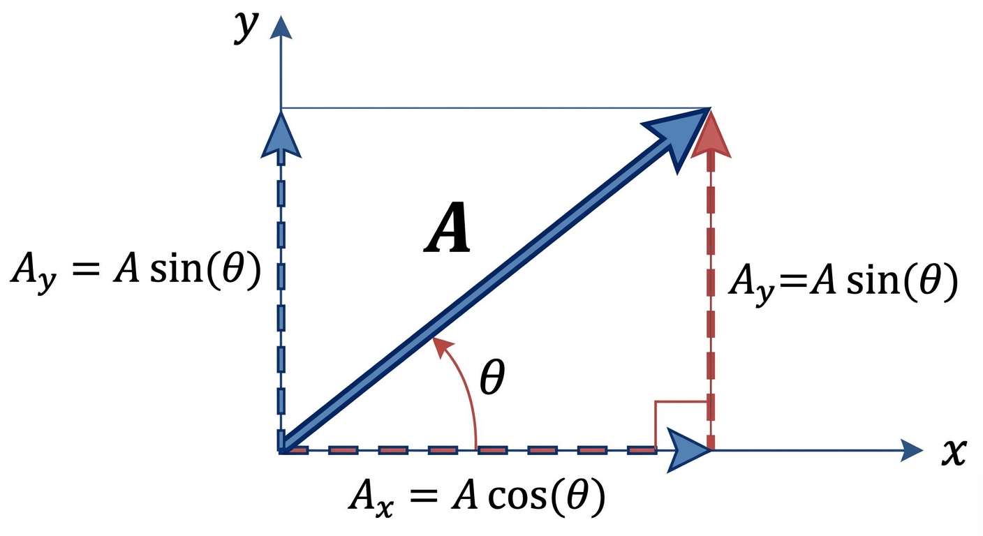
In two or three dimensions, vectors are often decomposed into components along the Cartesian axes ($x, y, z$). We use unit vectors to represent directions along the $x, y,$ and $z$ axes respectively.
For a position vector :
Key Vector Operations:
- Magnitude:
- Direction (Angle): (Be mindful of the quadrant!)
- Addition:
2. Motion in One Dimension: The Calculus Approach
In AP Physics C, kinematic variables are functions of time. You must be comfortable moving between position ($x$), velocity ($v$), and acceleration ($a$) using derivatives and integrals.
Position, Displacement, and Distance
- Position ($x(t)$): The coordinate location of a particle at time $t$.
- Displacement (): The vector change in position.
- Distance: The total scalar path length. This is the integral of speed.
Instantaneous vs. Average Velocity
- Average Velocity: depends only on endpoints.
- Instantaneous Velocity: The limit as time approaches zero; the derivative of position.
Example Problem:
An object moves such that its position is $x(t) = 4t^2 - 3t + 2$. Find its instantaneous velocity at $t=2$s.
Solution:
.
At $t=2$: .
Instantaneous vs. Average Acceleration
- Average Acceleration:
- Instantaneous Acceleration: The derivative of velocity (second derivative of position).
Moving "Backwards" with Integration
If you are given acceleration and asked for velocity, or velocity and asked for position, you must integrate. Don't forget the constant of integration ($+C$), which represents initial conditions ($v0$ or $x0$).
3. Uniformly Accelerated Motion (Constant Acceleration)
When acceleration is constant (constant magnitude and direction), the calculus definitions simplify into the "Big Five" algebraic equations. These are the workhorses for free-fall problems and simple dynamics.
The "Big Five" Kinematic Equations
| Equation | Missing Variable | application |
|---|---|---|
| $vx = v{x0} + a_xt$ | Velocity as a function of time | |
| $v_f$ | Position as a function of time | |
| $vx^2 = v{x0}^2 + 2ax(x - x0)$ | $t$ | Velocity as a function of position |
| $a$ | Average velocity displacement | |
| $v_0$ | Motion calculated from final velocity |
Free Fall
- Definition: An object moving solely under the influence of gravity.
- Condition: $a_y = -g$ (where ).
- Air Resistance: In Unit 1 problems, unless specified, ignore air resistance. (Drag forces are covered in Unit 2).
Common Trap: At the peak of a tossed object's flight, velocity is zero, but acceleration is still gravity (). Acceleration does not vanish just because the object stops momentarily.
4. Graphical Analysis of Motion
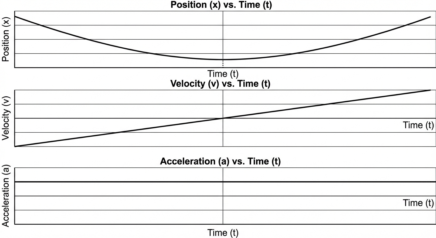
Interpreting graphs is a critical skill for the AP exam. The relationship between graphs mirrors the calculus relationships.
Relationship Table
| Graph Type | Slope Represents | Area Under Curve Represents |
|---|---|---|
| Position vs. Time ($x-t$) | Velocity ($v$) | N/A (physically meaningless) |
| Velocity vs. Time ($v-t$) | Acceleration ($a$) | Displacement () |
| Acceleration vs. Time ($a-t$) | Jerk (rate of change of $a$) | Change in Velocity () |
Visual Check:
- If $x-t$ is a parabola (degree 2), $v-t$ is a straight line (degree 1), and $a-t$ is a horizontal line (degree 0).
- Concavity: On an $x-t$ graph, concave up means positive acceleration ($a > 0$); concave down means negative acceleration ($a < 0$).
5. Motion in Two Dimensions
5.1 Projectile Motion
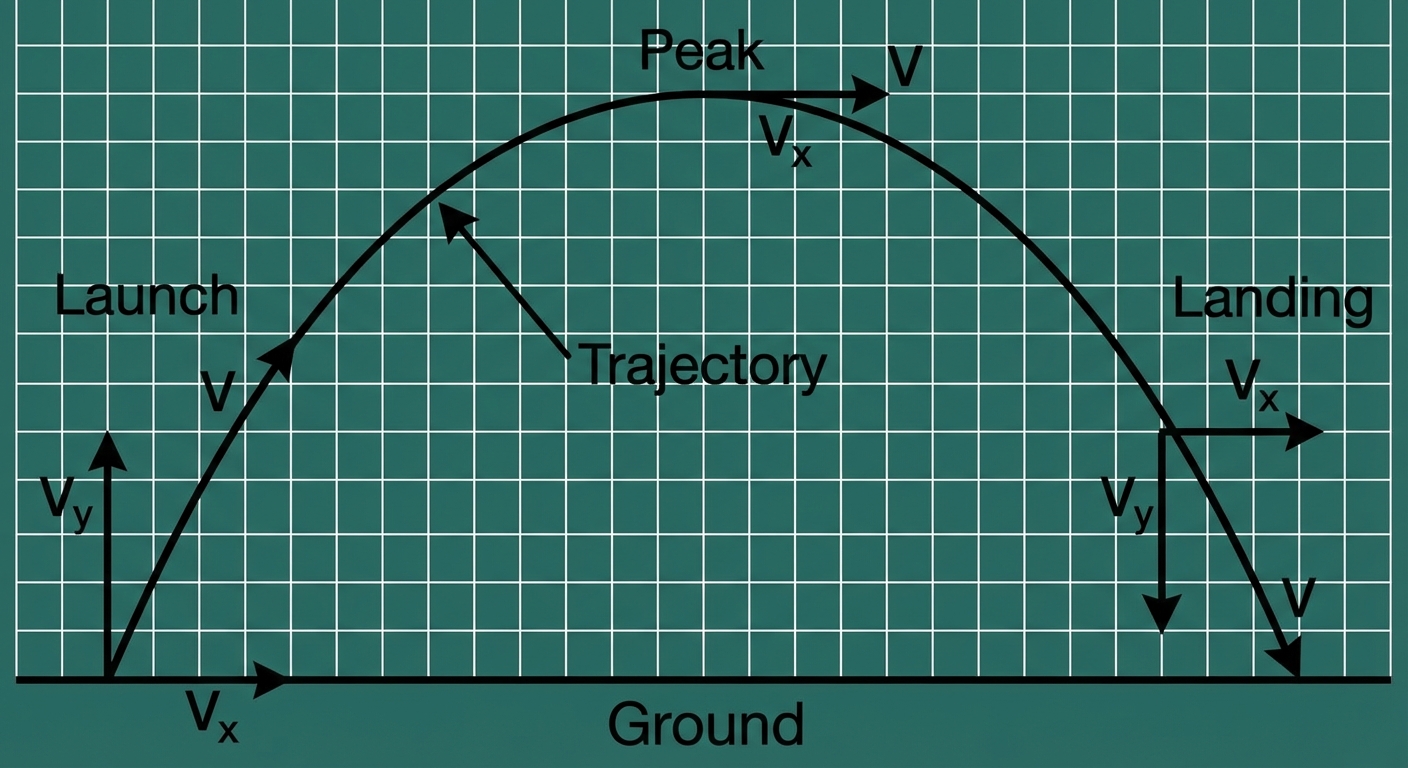
The key concept in 2D kinematics is the Independence of Perpendicular Motions. Motion in the $x$-direction is independent of motion in the $y$-direction. They are linked only by time ($t$).
Standard Analysis Setup:
| Axis | Acceleration | Velocity Equation | Position Equation |
|---|---|---|---|
| Horizontal ($x$) | $a_x = 0$ | (Constant) | |
| Vertical ($y$) | $a_y = -g$ |
The Range Equation (Special Case):
Only valid if the projectile lands at the same height it was launched:
Maximum range occurs at .
5.2 Relative Motion
Velocity is relative to the frame of reference. We use standard subscript notation:
- : Velocity of object A relative to C.
- : Velocity of object A relative to B.
- : Velocity of object B relative to C.
Vector Addition Rule:
mnemonic: The inner subscripts "match" and cancel out (B).
Example: A boat crosses a river.
- : Velocity of Boat relative to Water (engine speed).
- : Velocity of Water relative to Earth (river current).
- : Resultant velocity of Boat relative to Earth.
6. Common Mistakes & Pitfalls
Confusing Distance and Displacement:
- Running a lap around a 400m track: Distance = 400m, Displacement = 0.
- Integrals: is displacement; is magnitude of distance.
Sign Errors in Free Fall:
- Always define your coordinate system first (usually Up = positive). If Up is positive, $a = -9.8$. If Down is positive, $a = +9.8$.
- Make sure explicit velocities match signs (e.g., if throwing a ball down, $v_0$ is negative).
Misinterpreting Graphs:
- Thinking the intersection of two lines on a $v-t$ graph means the cars are colliding. (It just means they have the same speed; collisions happen when position lines intersect).
Mixing Axes in Projectiles:
- Using $v_y$ to calculate horizontal distance, or using $g$ in the $x$-equation. Keep your x and y tables completely separate until you solve for $t$.